
17 Exposure response analysis
17.1 Logistic regression
The use of logistic regression type of analyses is fairly common within exposure-response assessments. IQR Tools provides some functionality to quickly get results.
In this example, a dataset is provided, containing information about the occurrence of an adverse event (AE 1: yes, 0:no), a continuous predictor variable (AUC) and a categorical predictor variable (SEX). For each subject a single row in the dataset is provided. A subject is defined by the entry in the column ID.
# Load the AE analysis dataset
data <- IQRloadCSVdata("material/01-09-X1-LogisticRegression/dataAE.csv")| ID | AE | AETIME | AECENS | AUC | SEX |
|---|---|---|---|---|---|
| 1 | 0 | 44 | 1 | 50.73 | 1 |
| 2 | 0 | 119 | 1 | 31.39 | 1 |
| 3 | 0 | 75 | 1 | 76.30 | 1 |
| 4 | 1 | 50 | 0 | 271.04 | 0 |
| 5 | 1 | 41 | 0 | 150.33 | 0 |
| 6 | 0 | 135 | 1 | 44.64 | 1 |
| 7 | 1 | 36 | 0 | 568.08 | 1 |
| 8 | 0 | 218 | 1 | 74.50 | 1 |
| 9 | 1 | 10 | 0 | 760.56 | 1 |
| 10 | 0 | 61 | 1 | 287.74 | 1 |
17.1.1 Single predictor
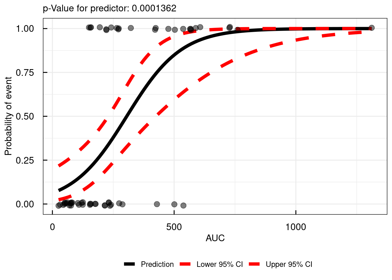
The function simple_IQRlogisticRegression() can be used to perform a logistic regression with respect to a single predictor variable. The names of the column, defining if an event has happened (AE) or not needs to be passed by the VARcol argument and the name of the column with the predictor variable (AUC) as the PREDcol argument.
The output of this function is a ggplot object.
# Simple logistic regression
simple_IQRlogisticRegression(
  data         = data,
  VARcol       = "AE",
  PREDcol      = "AUC"
)
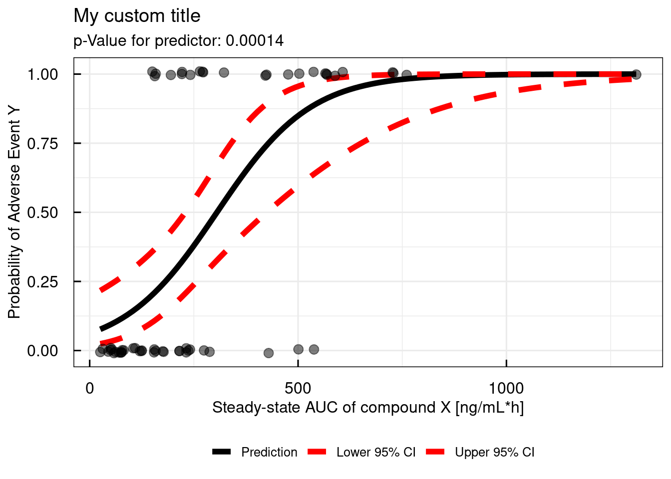
For report ready plots, the function allows to customize the annotation. An example is shown below:
# Simple logistic regression - add some annotation
simple_IQRlogisticRegression(
  data         = data,
  VARcol       = "AE",
  PREDcol      = "AUC",
  title        = "My custom title",
  xlab         = "Steady-state AUC of compound X [ng/mL*h]",
  ylab         = "Probability of Adverse Event Y",
  SIGNIF       = 2
)
17.2 Kaplan-Meier
Non-parametric survival analysis, using Kaplan Meier plots, is an often used technique for assessment of time-to-event data.
In this example, a dataset is provided, containing information about the occurrence of an adverse event (AE 1: yes, 0:no), the AETIME column represents the time at which an event has occurred (if AE=1) and the maximum observation period (if AE=0) during which the event has not occurred. The AECENS is the inverse of the AE column, providing information if the observation is censored (AECENS=1) or not (AECENS=0). An event is censored if it has not occurred during the observation period In addition the dataset contains a continuous predictor variable (AUC) and a categorical predictor variable (SEX). For each subject a single row in the dataset is provided. A subject is defined by the entry in the column ID.
For the Kaplan Meier analysis with IQR Tools either the event column (in the example: AE) or the censoring column (in the example: AECENS) can be used.
# Load the AE analysis dataset
data <- IQRloadCSVdata("material/01-09-X1-LogisticRegression/dataAE.csv")| ID | AE | AETIME | AECENS | AUC | SEX |
|---|---|---|---|---|---|
| 1 | 0 | 44 | 1 | 50.73 | 1 |
| 2 | 0 | 119 | 1 | 31.39 | 1 |
| 3 | 0 | 75 | 1 | 76.30 | 1 |
| 4 | 1 | 50 | 0 | 271.04 | 0 |
| 5 | 1 | 41 | 0 | 150.33 | 0 |
| 6 | 0 | 135 | 1 | 44.64 | 1 |
| 7 | 1 | 36 | 0 | 568.08 | 1 |
| 8 | 0 | 218 | 1 | 74.50 | 1 |
| 9 | 1 | 10 | 0 | 760.56 | 1 |
| 10 | 0 | 61 | 1 | 287.74 | 1 |
17.2.1 Simple plot
The function to generate a Kaplan Meier plot in IQR Tools is km_IQRsurvival(). The minimum required input arguments are
data, TIMEcol, and EVENTcol or CENScol. In the following examples we will mainly use the EVENTcol which codes for an event that happened during observation period with 1 and 0 for a no-event.
The function returns a list of two objects. The $plot object is a ggplot object with the Kaplan Meier plot. The $table object is an IQRoutputTable object that contains tabular information about the median survival time.
## $plot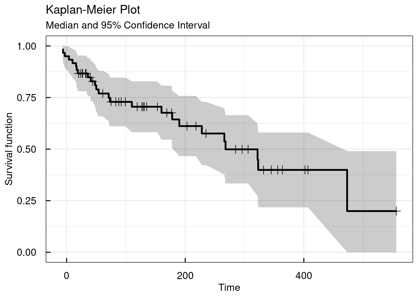
##
## $table
##    Strata   | Median Survival Time | 95% Confidence Interval
##    ---------------------------------------------------------
##    All data | 268                  | [190, 473]
##    ---------------------------------------------------------
## Number of significant digits: 4
##
## IQRoutputTable object
## $tableQuantiles
## NULL
##
## $tableCox
## NULL
The type argument allows to plot the lifetime distribution function instead of the survival curve.
# Simple KM plot - lifetime distribution function
km_IQRsurvival(
  data         = data,
  TIMEcol      = "AETIME",
  EVENTcol     = "AE",
  type         = "cdf"
)
## $plot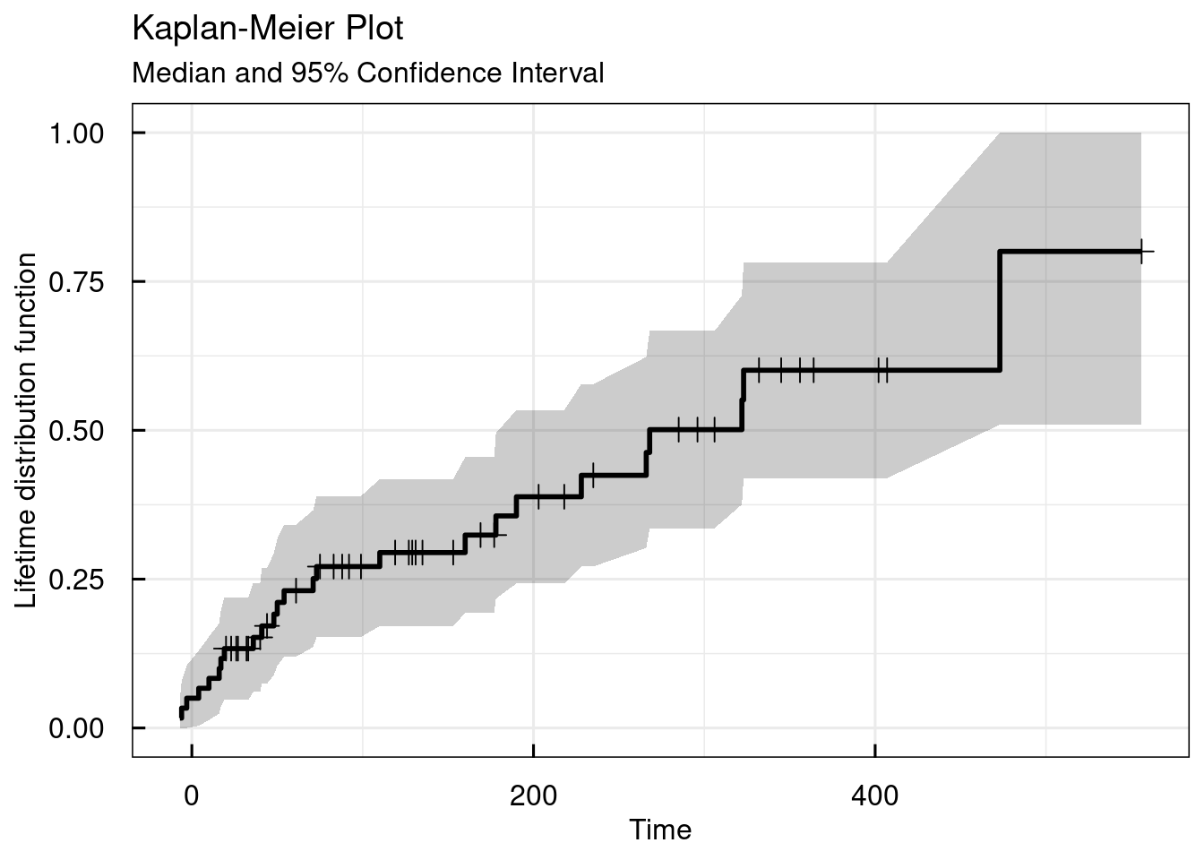
##
## $table
##    Strata   | Median Survival Time | 95% Confidence Interval
##    ---------------------------------------------------------
##    All data | 268                  | [190, 473]
##    ---------------------------------------------------------
## Number of significant digits: 4
##
## IQRoutputTable object
## $tableQuantiles
## NULL
##
## $tableCox
## NULL
17.2.2 Stratified plot
Using the STRATAcat argument, the Kaplan Meier plot can be stratified by a categorical variable in the dataset. Here
we use the column SEX as example:
# Simple KM survival plot - stratified by SEX
km_IQRsurvival(
  data         = data,
  TIMEcol      = "AETIME",
  EVENTcol     = "AE",
  STRATAcat    = "SEX"
)
## $plot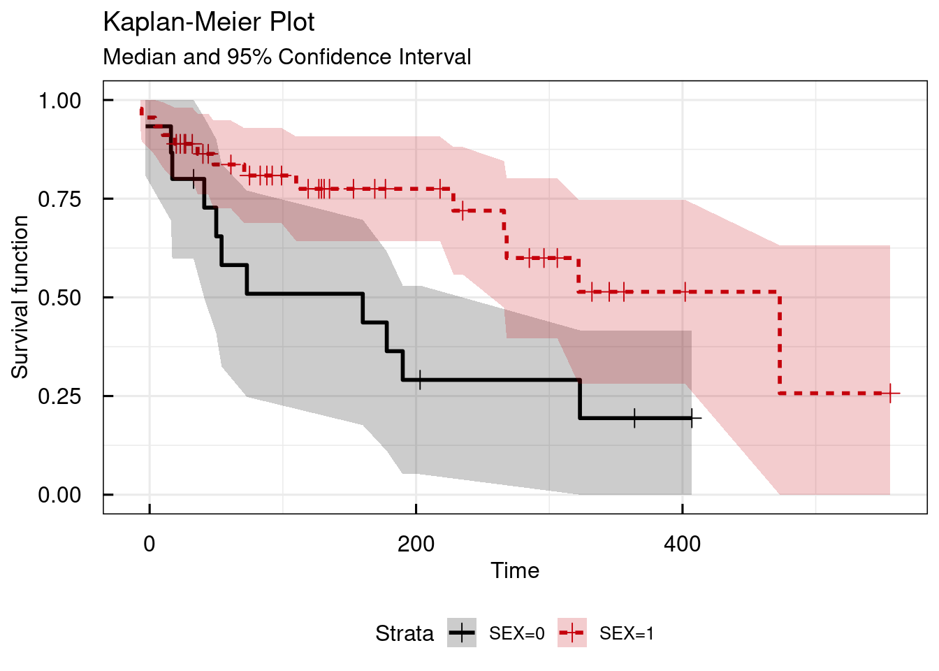
##
## $table
##    Strata | Median Survival Time | 95% Confidence Interval
##    -------------------------------------------------------
##    SEX=0  | 160                  | [41, 323]
##    SEX=1  | 473                  | [266, NA]
##    -------------------------------------------------------
## Number of significant digits: 4
##
## IQRoutputTable object
## $tableQuantiles
## NULL
##
## $tableCox
##    Result of cox regression for provided predictors
##    ==============================================================
##
##    PREDICTOR | COEF   | EXP.COEF. | SE.COEF. | P       | P_PHTEST
##    --------------------------------------------------------------
##    SEX1      | -0.965 | 0.381     | 0.4112   | 0.01895 | 0.8655
##    --------------------------------------------------------------
## survival::coxph(data=data,formula = dataKM~SEX)
## Number of significant digits: 4
## P: p-value defining statistical significance level of predictor variable
## P_PHTEST: p-value from the proportional hazard assumptions test (survival::cox.zph) of the cox regression (p>0.05: PH assumption valid)
##
## IQRoutputTable object
Using the STRATAcov argument, the Kaplan Meier plot can be stratified by a continuous variable in the dataset. Here
we use the column AUC as example. The argument probs.cont can be used to define in how many categories the continuous
covariate should be split. The defaul of 0.5 indicates that the median of AUC is used for stratification in this example.
# Simple KM survival plot - stratified by median of AUC
km_IQRsurvival(
  data         = data,
  TIMEcol      = "AETIME",
  EVENTcol     = "AE",
  STRATAcont   = "AUC",
  probs.cont   = 0.5
)
## $plot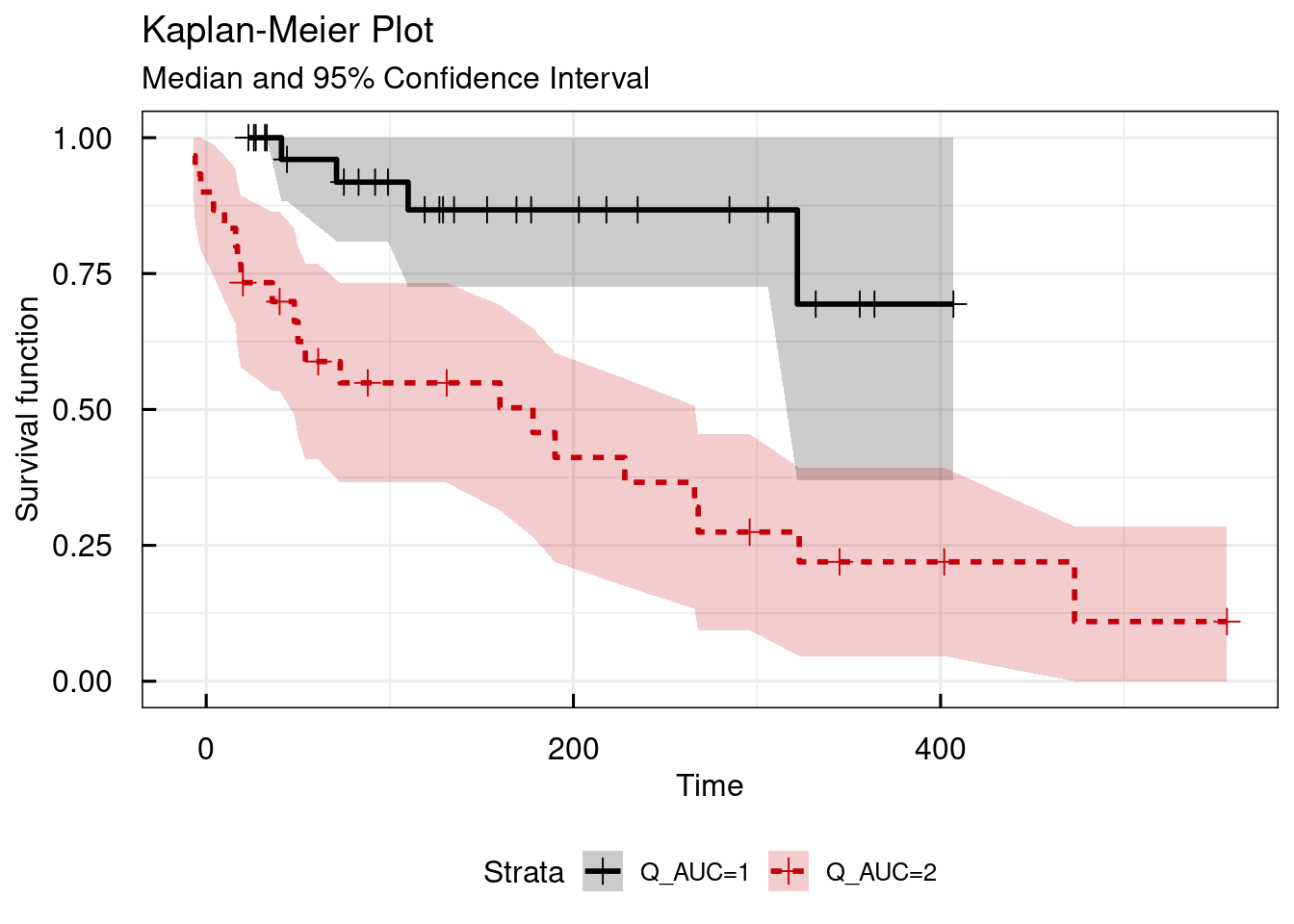
##
## $table
##    Strata  | Median Survival Time | 95% Confidence Interval
##    --------------------------------------------------------
##    Q_AUC=1 | NA                   | [322, NA]
##    Q_AUC=2 | 178                  | [48, 268]
##    --------------------------------------------------------
## Number of significant digits: 4
##
## IQRoutputTable object
## $tableQuantiles
##    Numeric values of quantile ranges
##    =====================================
##
##    VAR | Q1            | Q2
##    -------------------------------------
##    AUC | [25.37,218.3) | [218.3,1311.46]
##    -------------------------------------
## Used quantiles: [0.5]
## Number of significant digits: 4
##
## IQRoutputTable object
## $tableCox
##    Result of cox regression for provided predictors
##    ==============================================================
##
##    PREDICTOR | COEF  | EXP.COEF. | SE.COEF. | P        | P_PHTEST
##    --------------------------------------------------------------
##    Q_AUC2    | 1.735 | 5.667     | 0.5488   | 0.001574 | 0.2775
##    --------------------------------------------------------------
## survival::coxph(data=data,formula = dataKM~Q_AUC)
## Number of significant digits: 4
## P: p-value defining statistical significance level of predictor variable
## P_PHTEST: p-value from the proportional hazard assumptions test (survival::cox.zph) of the cox regression (p>0.05: PH assumption valid)
##
## IQRoutputTable object
Stratification by tertiles of the continuous variable (here: AUC) can be done in the following way:
# Simple KM survival plot - stratified by tertiles of AUC
km_IQRsurvival(
  data         = data,
  TIMEcol      = "AETIME",
  EVENTcol     = "AE",
  STRATAcont   = "AUC",
  probs.cont   = c(0.333,0.666)
)
## $plot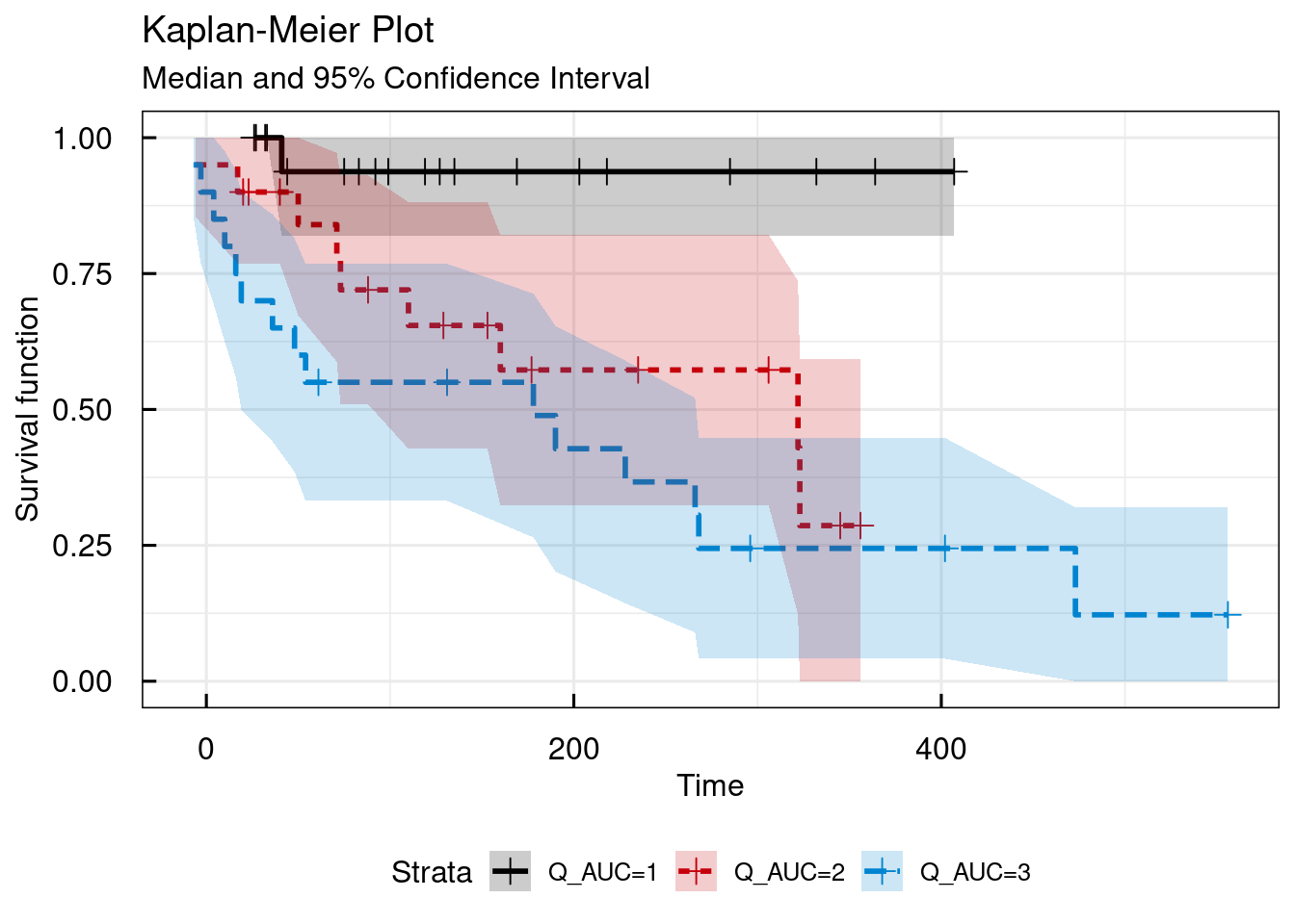
##
## $table
##    Strata  | Median Survival Time | 95% Confidence Interval
##    --------------------------------------------------------
##    Q_AUC=1 | NA                   | [NA, NA]
##    Q_AUC=2 | 322                  | [110, NA]
##    Q_AUC=3 | 178                  | [19, 268]
##    --------------------------------------------------------
## Number of significant digits: 4
##
## IQRoutputTable object
## $tableQuantiles
##    Numeric values of quantile ranges
##    =================================================
##
##    VAR | Q1          | Q2          | Q3
##    -------------------------------------------------
##    AUC | [25.37,153) | [153,272.9) | [272.9,1311.46]
##    -------------------------------------------------
## Used quantiles: [0.333,0.666]
## Number of significant digits: 4
##
## IQRoutputTable object
## $tableCox
##    Result of cox regression for provided predictors
##    ==============================================================
##
##    PREDICTOR | COEF  | EXP.COEF. | SE.COEF. | P        | P_PHTEST
##    --------------------------------------------------------------
##    Q_AUC2    | 2.165 | 8.717     | 1.054    | 0.04001  | 0.5025
##    Q_AUC3    | 2.67  | 14.44     | 1.036    | 0.009976 | 0.5025
##    --------------------------------------------------------------
## survival::coxph(data=data,formula = dataKM~Q_AUC)
## Number of significant digits: 4
## P: p-value defining statistical significance level of predictor variable
## P_PHTEST: p-value from the proportional hazard assumptions test (survival::cox.zph) of the cox regression (p>0.05: PH assumption valid)
##
## IQRoutputTable object
17.2.3 Style and annotation
If shaded confidence intervals are not desirable, these can be replaced by lines, using the shadedCI=FALSE argument:
# Simple KM survival plot - lines as CIs
km_IQRsurvival(
  data         = data,
  TIMEcol      = "AETIME",
  EVENTcol     = "AE",
  STRATAcont   = "AUC",
  probs.cont   = c(0.333,0.666),
  shadedCI     = FALSE
)
## $plot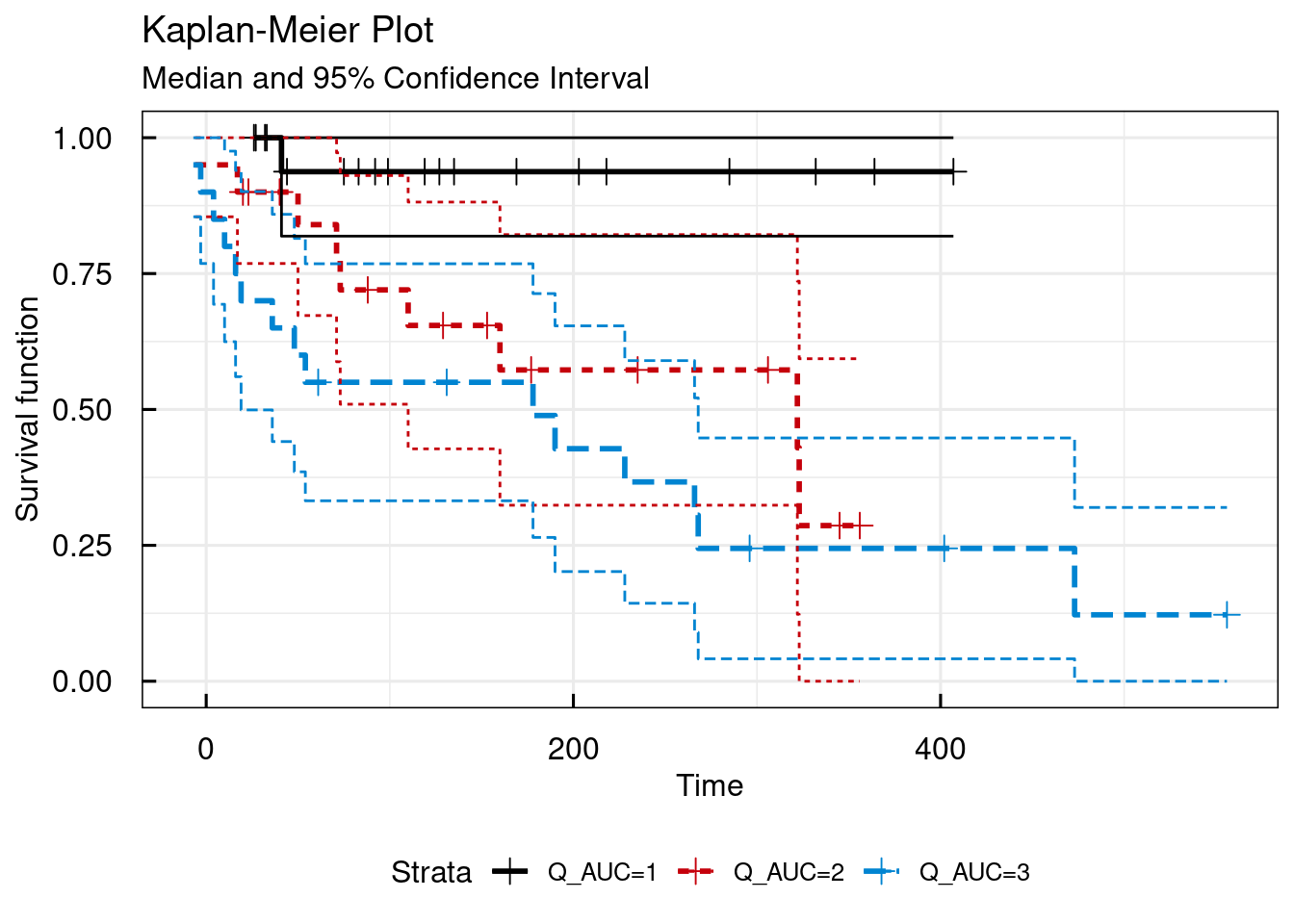
##
## $table
##    Strata  | Median Survival Time | 95% Confidence Interval
##    --------------------------------------------------------
##    Q_AUC=1 | NA                   | [NA, NA]
##    Q_AUC=2 | 322                  | [110, NA]
##    Q_AUC=3 | 178                  | [19, 268]
##    --------------------------------------------------------
## Number of significant digits: 4
##
## IQRoutputTable object
## $tableQuantiles
##    Numeric values of quantile ranges
##    =================================================
##
##    VAR | Q1          | Q2          | Q3
##    -------------------------------------------------
##    AUC | [25.37,153) | [153,272.9) | [272.9,1311.46]
##    -------------------------------------------------
## Used quantiles: [0.333,0.666]
## Number of significant digits: 4
##
## IQRoutputTable object
## $tableCox
##    Result of cox regression for provided predictors
##    ==============================================================
##
##    PREDICTOR | COEF  | EXP.COEF. | SE.COEF. | P        | P_PHTEST
##    --------------------------------------------------------------
##    Q_AUC2    | 2.165 | 8.717     | 1.054    | 0.04001  | 0.5025
##    Q_AUC3    | 2.67  | 14.44     | 1.036    | 0.009976 | 0.5025
##    --------------------------------------------------------------
## survival::coxph(data=data,formula = dataKM~Q_AUC)
## Number of significant digits: 4
## P: p-value defining statistical significance level of predictor variable
## P_PHTEST: p-value from the proportional hazard assumptions test (survival::cox.zph) of the cox regression (p>0.05: PH assumption valid)
##
## IQRoutputTable object
To allow for report ready annotation of plots, several additional arguments are available (legend.labs, title, xlab, ylab):
# Simple KM survival plot - change annotation
km_IQRsurvival(
  data         = data,
  TIMEcol      = "AETIME",
  EVENTcol     = "AE",
  STRATAcont   = "AUC",
  probs.cont   = c(0.333,0.666),
  shadedCI     = FALSE,
  legend.labs  = c("AUC Tertile 1", "AUC Tertile 2", "AUC Tertile 3"),
  title        = "My custom title for this plot",
  xlab         = "Time since first dose [Days]",
  ylab         = ""
)
## $plot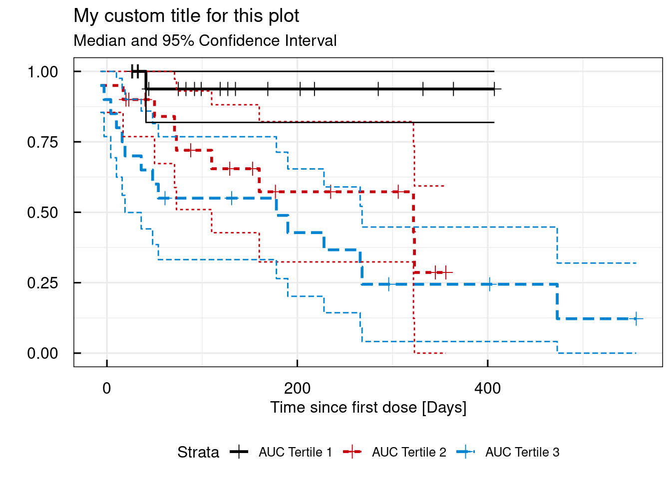
##
## $table
##    Strata        | Median Survival Time | 95% Confidence Interval
##    --------------------------------------------------------------
##    AUC Tertile 1 | NA                   | [NA, NA]
##    AUC Tertile 2 | 322                  | [110, NA]
##    AUC Tertile 3 | 178                  | [19, 268]
##    --------------------------------------------------------------
## Number of significant digits: 4
##
## IQRoutputTable object
## $tableQuantiles
##    Numeric values of quantile ranges
##    =================================================
##
##    VAR | Q1          | Q2          | Q3
##    -------------------------------------------------
##    AUC | [25.37,153) | [153,272.9) | [272.9,1311.46]
##    -------------------------------------------------
## Used quantiles: [0.333,0.666]
## Number of significant digits: 4
##
## IQRoutputTable object
## $tableCox
##    Result of cox regression for provided predictors
##    ==============================================================
##
##    PREDICTOR | COEF  | EXP.COEF. | SE.COEF. | P        | P_PHTEST
##    --------------------------------------------------------------
##    Q_AUC2    | 2.165 | 8.717     | 1.054    | 0.04001  | 0.5025
##    Q_AUC3    | 2.67  | 14.44     | 1.036    | 0.009976 | 0.5025
##    --------------------------------------------------------------
## survival::coxph(data=data,formula = dataKM~Q_AUC)
## Number of significant digits: 4
## P: p-value defining statistical significance level of predictor variable
## P_PHTEST: p-value from the proportional hazard assumptions test (survival::cox.zph) of the cox regression (p>0.05: PH assumption valid)
##
## IQRoutputTable object
17.2.4 Risk table
A risk table can be added below the KM plot by setting the argument risk.table to TRUE.
The risk table reports how many subjects at a given time still are at risk to have an even to observed.
# Simple KM survival plot - add an "at risk" table
km_IQRsurvival(
  data         = data,
  TIMEcol      = "AETIME",
  EVENTcol     = "AE",
  STRATAcont   = "AUC",
  probs.cont   = c(0.333,0.666),
  shadedCI     = FALSE,
  legend.labs  = c("AUC Tertile 1", "AUC Tertile 2", "AUC Tertile 3"),
  title        = "My custom title for this plot",
  xlab         = "Time since first dose [Days]",
  ylab         = "",
  risk.table   = TRUE
)
## $plot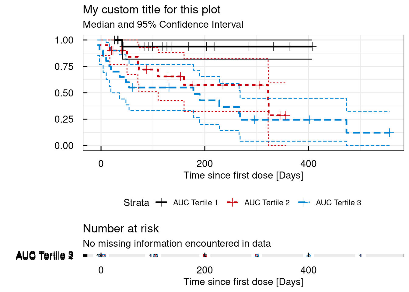
##
## $table
##    Strata        | Median Survival Time | 95% Confidence Interval
##    --------------------------------------------------------------
##    AUC Tertile 1 | NA                   | [NA, NA]
##    AUC Tertile 2 | 322                  | [110, NA]
##    AUC Tertile 3 | 178                  | [19, 268]
##    --------------------------------------------------------------
## Number of significant digits: 4
##
## IQRoutputTable object
## $tableQuantiles
##    Numeric values of quantile ranges
##    =================================================
##
##    VAR | Q1          | Q2          | Q3
##    -------------------------------------------------
##    AUC | [25.37,153) | [153,272.9) | [272.9,1311.46]
##    -------------------------------------------------
## Used quantiles: [0.333,0.666]
## Number of significant digits: 4
##
## IQRoutputTable object
## $tableCox
##    Result of cox regression for provided predictors
##    ==============================================================
##
##    PREDICTOR | COEF  | EXP.COEF. | SE.COEF. | P        | P_PHTEST
##    --------------------------------------------------------------
##    Q_AUC2    | 2.165 | 8.717     | 1.054    | 0.04001  | 0.5025
##    Q_AUC3    | 2.67  | 14.44     | 1.036    | 0.009976 | 0.5025
##    --------------------------------------------------------------
## survival::coxph(data=data,formula = dataKM~Q_AUC)
## Number of significant digits: 4
## P: p-value defining statistical significance level of predictor variable
## P_PHTEST: p-value from the proportional hazard assumptions test (survival::cox.zph) of the cox regression (p>0.05: PH assumption valid)
##
## IQRoutputTable object
17.2.5 Confidence intervals
The width of the confidence intervals can be selected using the conf.int argument:
# Simple KM survival plot - different confidence interval setting
km_IQRsurvival(
  data         = data,
  TIMEcol      = "AETIME",
  EVENTcol     = "AE",
  STRATAcont   = "AUC",
  probs.cont   = c(0.333,0.666),
  shadedCI     = TRUE,
  legend.labs  = c("AUC Tertile 1", "AUC Tertile 2", "AUC Tertile 3"),
  title        = "My custom title for this plot",
  xlab         = "Time since first dose [Days]",
  ylab         = "",
  risk.table   = TRUE,
  conf.int     = 0.8
)
## $plot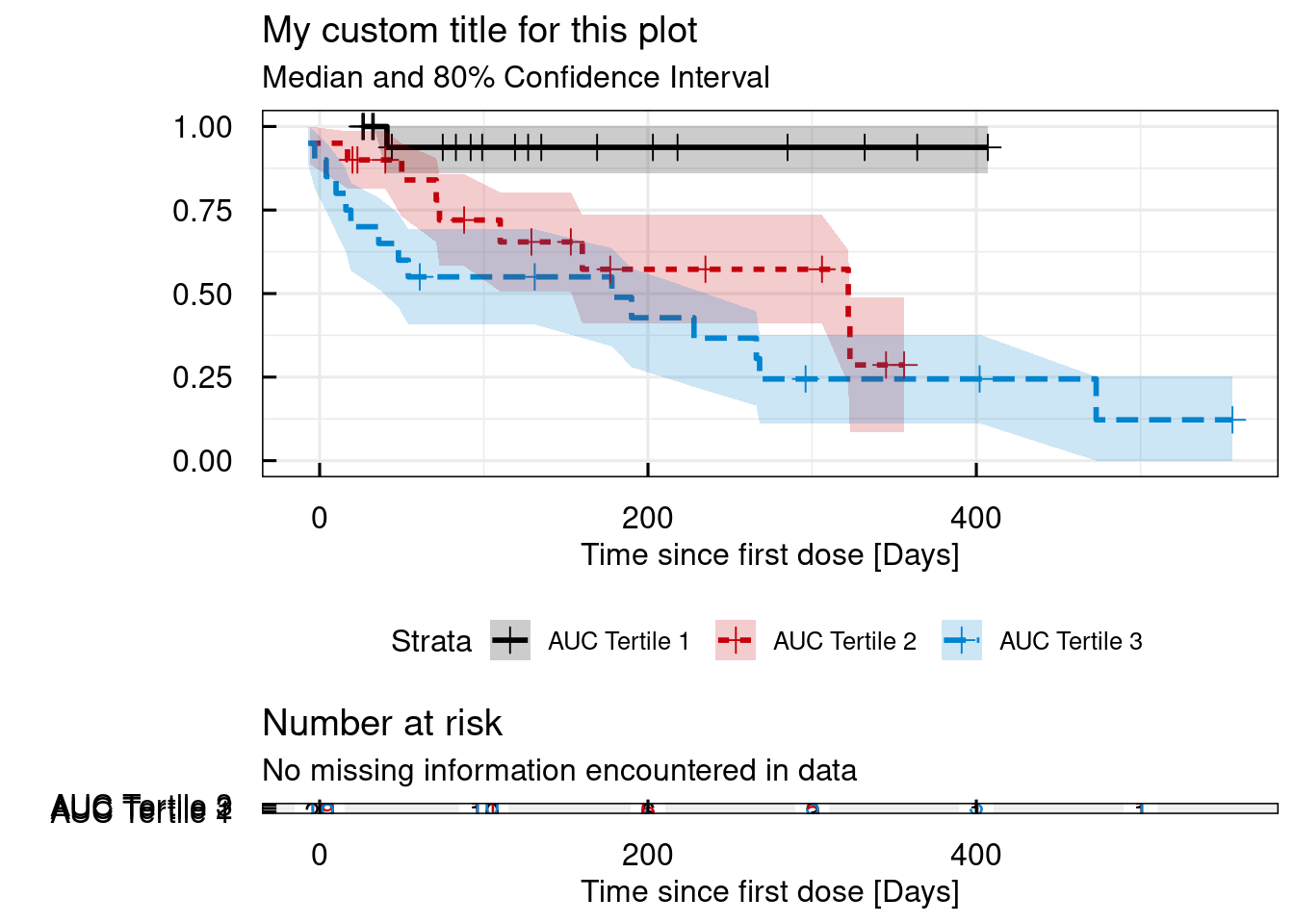
##
## $table
##    Strata        | Median Survival Time | 80% Confidence Interval
##    --------------------------------------------------------------
##    AUC Tertile 1 | NA                   | [NA, NA]
##    AUC Tertile 2 | 322                  | [160, 323]
##    AUC Tertile 3 | 178                  | [48, 266]
##    --------------------------------------------------------------
## Number of significant digits: 4
##
## IQRoutputTable object
## $tableQuantiles
##    Numeric values of quantile ranges
##    =================================================
##
##    VAR | Q1          | Q2          | Q3
##    -------------------------------------------------
##    AUC | [25.37,153) | [153,272.9) | [272.9,1311.46]
##    -------------------------------------------------
## Used quantiles: [0.333,0.666]
## Number of significant digits: 4
##
## IQRoutputTable object
## $tableCox
##    Result of cox regression for provided predictors
##    ==============================================================
##
##    PREDICTOR | COEF  | EXP.COEF. | SE.COEF. | P        | P_PHTEST
##    --------------------------------------------------------------
##    Q_AUC2    | 2.165 | 8.717     | 1.054    | 0.04001  | 0.5025
##    Q_AUC3    | 2.67  | 14.44     | 1.036    | 0.009976 | 0.5025
##    --------------------------------------------------------------
## survival::coxph(data=data,formula = dataKM~Q_AUC)
## Number of significant digits: 4
## P: p-value defining statistical significance level of predictor variable
## P_PHTEST: p-value from the proportional hazard assumptions test (survival::cox.zph) of the cox regression (p>0.05: PH assumption valid)
##
## IQRoutputTable object
17.2.6 Using the CENScol argument
In the previous examples the column in the dataset that defined if an event had been observed (1) or not (0) was used by defining the EVENTcol argument as the name of the corresponding colmn (AE) in the dataset. In the following example, instead of the event column the censoring column (AECENS) is used and passed to the function as the CENScol argument. The results will be identical as in the first example above. It should be clear that in the same function call only one of the two arguments (EVENTcol or CENScol) are allowed to be defined.
## $plot
##
## $table
##    Strata   | Median Survival Time | 95% Confidence Interval
##    ---------------------------------------------------------
##    All data | 268                  | [190, 473]
##    ---------------------------------------------------------
## Number of significant digits: 4
##
## IQRoutputTable object
## $tableQuantiles
## NULL
##
## $tableCox
## NULL
All the other examples as for EVENTcol apply in the same way to the case where CENScol is used instead.