
11 NLME Modeling
Non linear mixed effects (NLME) modeling is a standard method for pharmacometric analyses. In mixed effects modeling, fixed effects include the average parameters of the population and covariates, whereas the random effects account for residual random variability between individuals. Inter-individual variability is quantified and its dependence on covariates is assessed.
To date, there are two major platforms for NLME modeling: NONMEM and MONOLIX. Often, users are faced with the decision which platform to use or are missing the training to make optimal use of both platforms. In the following, a novel approach to NLME modeling is explained, which concentrates on making modeling more user-friendly and accessible by shifting the focus from the software to modeling. This is achieved by providing a software framework (IQR Tools), that gives the opportunity to change freely between NONMEM and MONOLIX and presents the results in a humanly understandable way.
Recently NLMIXR has stepped onto the scene of NLME parameter estimation tools. It is still in its infancy but developing quickly. And it is open source! IQR Tools interfaces to NLMIXR just as it interfaces to NONMEM and MONOLIX and provides the user with a seamless experience of using it.
The present chapter discusses three main types of NLME model:
- Longitudinal models: General longitudinal NLME models with one or more dosing inputs and one or more observe variables. This includes, but it not limited to, typical PK and joint PKPD models. The main important thing is that models need to be representable by ordinary differential equations.
- Time to event models: Fully parameteric time-to-event models. IQR Tools allows to generate model for a wide range of survival data distributions.
- Joint models: Mixed longitudinal and event models. For example useful when a hazard function for an event (e.g. overall survival) is to be informed by a continuous varible in the model.
11.1 Longitudinal Models
The generation and execution of longitudinal NLME models is split into two main steps. The first step is to setup an NLME estimation object using the function IQRnlmeEst(). The second step is to generate an IQRnlmeProject based on the estimation object, using the IQRnlmeProject() function. Such a project can then be executed and further analyzed (see the Chapter about Model Evalution).
Information that is required for the setup of an NLME project are the following:
- Data
- Structural model
- Dosing information
- Model specification (e.g., initial guesses, statistical model, covariate model, error model, etc.)
11.1.1 Required data format
The data needs to be in IQRnlmeData format. The minimally required columns for this format are:
IXGDF: Index number for individual records in datasetUSUBJID: Unique subject identifier (across all records of a subject)ID: Modeling tool specific subject identifierTIME: Time point of event (observation or dosing)TIMEPOS: Time from first event in datasetTAD: Time passed since last doseYTYPE: Number of output observation linking model to data (0 for doses)DV: Value of the observation event (0 for doses)MDV: Missing data flag (1 for missing observations and dose records, 0 otherwise)EVID: Event ID (0 for observations, 1 for dosing records)CENS: Censoring flag (0 uncensored, 1 left censored)AMT: Dosing amount for dose event (otherwhise 0)ADM: Number of input for dose (otherwhise 0)RATE: Rate of administration if infusion (bolus: 0, estimated:-2)TINF: Infusion time - used for both NONMEM and MONOLIX. 0 if bolus, >0 if infusion. If infusion (or 0th order absorption) duration is selected to be estimated then the values in this column are neglected.YTYPE or CMT: If YTYPE: Number of output if observation, NA if dosing event. If CMT: Number of output if observation, number of state to which to add dose if dosing event.
Further columns containing information about covariates and regressors can be added as needed.
The IQRnlmeData format can be generated from IQRdataGeneral format by exporting the dataset as csv file with the function exportNLME_IQRdataGENERAL().
11.1.2 Structural models
Structural models are defined using the syntax of the IQRmodel object in IQR Tools. This is a ODE based format, described earlier in this book. An example for a simple structural PK/PD model based on Friberg et al. 2002 is shown below:
********** MODEL NAME
Neutropenia Model
********** MODEL NOTES
Example neutropenia model
Dose unit:    mg
Output unit : 10^9 cells/L
Time unit:    hours
********** MODEL STATES
# Differential equations PK model
d/dt(A_centr)  = - CL/Vc*A_centr - Q/Vc*A_centr + A_periph*Q/Vp + INPUT1
d/dt(A_periph) =                   Q/Vc*A_centr - A_periph*Q/Vp

# Differential equations Friberg model
d/dt(A_prol)   = KTR*A_prol*(1-SLOPU*CONC)*(CIRC0/A_circ)^GAM - KTR*A_prol
d/dt(A_tr1)    = KTR*A_prol - KTR*A_tr1
d/dt(A_tr2)    = KTR*A_tr1 - KTR*A_tr2
d/dt(A_tr3)    = KTR*A_tr2 - KTR*A_tr3
d/dt(A_circ)   = KTR*A_tr3 - KTR*A_circ

# Initial conditions
A_prol(0)      = CIRC0
A_tr1(0)       = CIRC0
A_tr2(0)       = CIRC0
A_tr3(0)       = CIRC0
A_circ(0)      = CIRC0
********** MODEL PARAMETERS
# Define parameters
CIRC0          =  7.21   # Baseline circulating neutrophils (10^9 cells/L)
MTT            =  124    # Mean transit time (hours)
SLOPU          =  28.9   # Slope of drug effect (mL/ug)
GAM            = 0.239   # Exponent (.)

# Define regression parameters
Vp             = 1    # Peripheral volume (L)
Vc             = 1    # Central volume (L)
CL             = 1    # Clearance (L/hour)
Q              = 1    # Intercompartmental clearance (L/hour)
********** MODEL VARIABLES
# Calculate central concentration
CONC           = A_centr/Vc

# PD parameters
KTR            = 4/MTT

# Output for fitting
OUTPUT1        = A_circ  # (10^9 cells/L) Circulating neutrophils
********** MODEL REACTIONS
********** MODEL FUNCTIONS
********** MODEL EVENTS
11.1.3 Linear vs. nonlinear models
In case that a structural model is linear, NONMEM, MONOLIX, and NLMIXR allow to specify the model in a special way (in NONMEM codes such as ADVAN 1, 2, 3, 4, 5, 7, 11, 12 are used) in order to ensure that the model does not need to be integrated and instead analytic or a matrix exponential approach is used. This speeds up the execution of an NLME model tremendously.
In IQR Tools a structural model is always defined in terms of its differential equations. Internally, IQR Tools will analyze the model and, in case it is linear, will use the appropriate coding of NONMEM and MONOLIX models to ensure the available analytic of matrix exponential solution is used. If the model is non-linear, IQR Tools will export the ODEs to NONMEM or MONOLIX or NLMIXR and integration of ODEs is used to solve the model.
11.1.4 Time varying covariates
IQR Tools by default uses the MU referencing (see for example here) for the implementation of parameter transformations and covariates. The use of MU referencing is important for better convergence of EM methods such as SAEM in both NONMEM and MONOLIX.
A drawback of MU referencing is that covariates implemented in this way need to be time independent. Even if they are coded in the dataset in a time dependent manner, only the first value will be considered by SAEM and thus in reality it will be turned into a time invariant covariate.
In order to implement time varying covariates, IQR Tools uses something called regression parameters. Each regression parameter is simply a column in the dataset with a name. This name can appear in a structural model as a parameter and will receive the values from the column in the dataset. No interpolation is done over time. Carry forward of the last value is used. For NONMEM users the difference to the typical implementation of time varying covariates might not be obvious - as all seems to be as always. MONOLIX users will recognize the term regression parameters.
Things to remember: When implementing time varying covariates in NLME models with IQR Tools, the respective columns need to be defined as regression parameters (we will see this in examples below). This is also possible in the case of time invariant covariates and complex covariate models that cannot be implemented using MU referencing.
11.1.5 Basic PK model
This first example is important as many concepts will be introduced. Following examples will then only focus on the things that can be done differently and not repeat the basics.
11.1.5.1 Data
An example dataset is provided in the material, based on the ubiquitous Theophylline dataset. A preview of the first 10 columns of this dataset is shown below:
| IXGDF | ID | USUBJID | TIME | TIMEPOS | TAD | TIMEUNIT | YTYPE | NAME | DV | UNIT | CENS | MDV | EVID | AMT | ADM | RATE | TINF | WT0 | SEX |
|---|---|---|---|---|---|---|---|---|---|---|---|---|---|---|---|---|---|---|---|
| 1 | 1 | Theo_1 | 0.00 | 0.00 | 0.00 | Hours | 0 | Dose | 0.00 | mg | 0 | 1 | 1 | 400 | 1 | 0 | 0 | 79.6 | 1 |
| 2 | 1 | Theo_1 | 0.25 | 0.25 | 0.25 | Hours | 1 | Concentration | 2.84 | ug/ml | 0 | 0 | 0 | 0 | 0 | 0 | 0 | 79.6 | 1 |
| 3 | 1 | Theo_1 | 0.57 | 0.57 | 0.57 | Hours | 1 | Concentration | 6.57 | ug/ml | 0 | 0 | 0 | 0 | 0 | 0 | 0 | 79.6 | 1 |
| 4 | 1 | Theo_1 | 1.12 | 1.12 | 1.12 | Hours | 1 | Concentration | 10.50 | ug/ml | 0 | 0 | 0 | 0 | 0 | 0 | 0 | 79.6 | 1 |
| 5 | 1 | Theo_1 | 2.02 | 2.02 | 2.02 | Hours | 1 | Concentration | 9.66 | ug/ml | 0 | 0 | 0 | 0 | 0 | 0 | 0 | 79.6 | 1 |
| 6 | 1 | Theo_1 | 3.82 | 3.82 | 3.82 | Hours | 1 | Concentration | 8.58 | ug/ml | 0 | 0 | 0 | 0 | 0 | 0 | 0 | 79.6 | 1 |
| 7 | 1 | Theo_1 | 5.10 | 5.10 | 5.10 | Hours | 1 | Concentration | 8.36 | ug/ml | 0 | 0 | 0 | 0 | 0 | 0 | 0 | 79.6 | 1 |
| 8 | 1 | Theo_1 | 7.03 | 7.03 | 7.03 | Hours | 1 | Concentration | 7.47 | ug/ml | 0 | 0 | 0 | 0 | 0 | 0 | 0 | 79.6 | 1 |
| 9 | 1 | Theo_1 | 9.05 | 9.05 | 9.05 | Hours | 1 | Concentration | 6.89 | ug/ml | 0 | 0 | 0 | 0 | 0 | 0 | 0 | 79.6 | 1 |
| 10 | 1 | Theo_1 | 12.12 | 12.12 | 12.12 | Hours | 1 | Concentration | 5.94 | ug/ml | 0 | 0 | 0 | 0 | 0 | 0 | 0 | 79.6 | 1 |
The function data_IQRest() is used to generate a list that specifies the data object to be used for the NLME model generation.
The only required argument to this function is data, which should be defined with the absolute or relative path to the dataset to be used for estimation. Optional arguments are covNames, catNames, and regressorNames.
data          <- data_IQRest(
  datafile       = "material/01-04a-X1-NLME/Ex1/data.csv",  # absolute or relative path to the dataset
  covNames       = c("WT0"),      # specifying continuos candidate covariates
  catNames       = c("SEX")       # vector with names of categorical covariates
)
covNames can be assigned a character vector, defining the candidate continuous covariates to be considered. The names provided in this vector need to be available in the dataset as column names. In a similar manner, catNames is used to define candidate categorical covariates.
regressorNames is used in the same manner to define potentially time varying columns in the dataset that are passed to the model as regression parameters. For traditional terminology, regression parameter are best understood as time varying covariates. See a discussion about this here.
The term candidate covariate does not mean that this covariate is automatically included into the model. Inclusion into the model has to be defined separately. But the presence of candidate covariates allows to generate diagnstics for these. In this example here the two candidate covariates WT (weight) and SEX (gender) are present in the data and will be defined. No regression parameter is present.
11.1.5.2 Structural model
A structural model is provided as an IQRmodel text file, coding for a one compartment model with first order absorption. The model can be seen here. The only thing to do with the model at this point is to load it into R as follows:
11.1.5.3 Dosing definition
Inspecting the structural model we see that it has one dosing input (INPUT1). For the setup of an estimation object information about the type of the input needs to be provided. Possible types are BOLUS, INFUSION, and ABSORPTION0. The main difference between INFUSION and ABSORPTION0 is that in the first case the infusion time is provided by the dataset and in the latter case the zero-order absorption duration is estimated.
The dosing information in this example is defined as follows:
For each input an argument with the name of the input needs to be provided, and the value or each argument is a vector with several optional arguments. The only required argument is the first with name type, defining the type of the administration (see above). Optional arguments are information about the names for zero-order absorption and lag time parameters. Theis use is shown in later examples.
11.1.5.4 Model specification
A model specification contains all information about fixed and random effect parameters, the error model, the covariance model, and covariate model that should be applied. It states, e.g., whether a parameter is estimated or should be fixed, specifies the distributions for the individual parameter, or implements a (time-independent) covariate on a parameter.
In this first an example, we build a model with no covariates or covariances between individual parameters. All the model specification information needs to be stored in a list with preserved field names. For convenience, we make use of the function modelSpec_IQRest() that accepts the preserved names as inputs and returns an appropriate list.
The following is an example for a minimally needed model specification list, defining only the initial guesses for the fixed effects to be estimated.
## Model specification
modelSpec     <- modelSpec_IQRest(
  # Defining the initial guesses for the fixed effect parameters
  POPvalues0  = c(CL=40, Vc=2, ka=2)
)
The modelSpec_IQRest() function has many optional arguments to allow detailed control over the NLME model to be built. In this minimal case, all fixed effects will be estimated, the distribution of the individual parameters is assumed to be lognormal, the initial guesses for the random effects if 0.5 (standard deviation), representing 50%CV. Furthermore, no covariates are used on the parameters, a diagonal random effect covariance matrix and an additive error model is used.
11.1.5.5 Estimation object
After definition of the above elements (data, model, dosing, and modelSpec), the IQRnlmeEst() function is used to generate an NLME estimation object.
## Building estimation object
est <- IQRnlmeEst(model         = model,
                  dosing        = dosing,
                  data          = data,
                  modelSpec     = modelSpec)
The ´´IQRnlmeEst()´´ function performs checks to assess if the different elements are compatible. For example whether covariates used in the model specification are contained the data or parameters to be estimates match the parameters of the structural model. The output of the function is a list in R with its own ``print()```function, displaying general information about the NLME estimation object that allows a modeler to check if the desired definitions have correctly been implemented.
##
## ==================================================================
## == IQRnlmeEst information
## ==================================================================
##
##    NLME data file: material/01-04a-X1-NLME/Ex1/data.csv
##
##
##    Summary of parameter estimation specification (parameters)
##    ========================================================================================================================================================================================
##
##    PARAMETER | INITIAL.GUESS.FIXED.EFFECT | IIV.IOV.DISTRIBUTION | INITIAL.GUESS.IIV.RANDOM.EFFECT | INITIAL.GUESS.IOV.RANDOM.EFFECT | FIXED.EFFECT | IIV.RANDOM.EFFECT | IOV.RANDOM.EFFECT
##    ----------------------------------------------------------------------------------------------------------------------------------------------------------------------------------------
##    ka        | 2                          | LogNormal            | 0.5                             | 0.5                             | ESTIMATED    | ESTIMATED         | NONE (kept on 0)
##    CL        | 40                         | LogNormal            | 0.5                             | 0.5                             | ESTIMATED    | ESTIMATED         | NONE (kept on 0)
##    Vc        | 2                          | LogNormal            | 0.5                             | 0.5                             | ESTIMATED    | ESTIMATED         | NONE (kept on 0)
##
##
## IQRoutputTable object
##
##    Regression parameters considered in the model:
##    ==============================================
##    No regression parameters considered.
##
##
##    Matching between data header names and identifiers
##    ==================================================
##
##    DATAHEADER | DATAHEADER.IDENT
##    --------------------------------------------------
##    IXGDF      | IGNORE
##    ID         | ID
##    USUBJID    | IGNORE
##    TIME       | TIME
##    TIMEPOS    | TIMEPOS
##    TAD        | TAD
##    TIMEUNIT   | IGNORE
##    YTYPE      | YTYPE
##    NAME       | IGNORE
##    DV         | DV
##    UNIT       | IGNORE
##    CENS       | CENS
##    MDV        | MDV
##    EVID       | EVID
##    AMT        | AMT
##    ADM        | ADM
##    RATE       | RATE
##    TINF       | TINF
##    WT0        | COV
##    SEX        | CAT
##
##
## IQRoutputTable object
##
##    Error model information
##    =============================================
##
##    OUTPUT  | ERROR.MODEL         | INITIAL.GUESS
##    ---------------------------------------------
##    OUTPUT1 | Absolute (Additive) | 1
##
##
## IQRoutputTable object
##    Covariate estimation information
##    ================================
##    No covariates considered.
##
##    The model is linear and can be solved analytically.
##    ===================================================
##      - In NONMEM ADVAN1,2,3,4,5,7,11, or 12 will be used, depending on the model structure.
##      - Please note that in MONOLIX an analytic solution can only be used if there is only one route of elimination.
##        Otherwise the model is integrated.
##      - Please ensure no constant zero order terms are entering ODE RHSs! These are unhandled and unchecked.
##        If such things are present, please use the ODE based solution for now.
##      - Using the analytic solution can be overriden by an input argument to IQRnlmeProject
##
##
## IQRnlmeEst object
11.1.5.6 NLME project
The NLME estimation object is still estimation tool independent. The next step in the NLME workflow is to generate a tool dependent NLME project. Currently supported tools are NONMEM, MONOLIX, and NLMIXR.
A tool dependent NLME project can be generated, using the function IQRnlmeProject(). Here in this example we will generate 2 identical NLME projects - one for NONMEM and one for MONOLIX. For the purpose of this doumentation, NLMIXR is not considered as installation of NLMIXR can be fairly cumbersome.
# Creating a NONMEM project
projNONMEM <- IQRnlmeProject(est = est,
                             projectPath="material/01-04a-X1-NLME/Ex1/NONMEM",
                             tool="NONMEM",
                             algOpt.K1 = 50,
                             algOpt.K2 = 20,
                             comment = "1 cpt model with 1st order absorption - NONMEM version")

# Creating a MONOLIX project
projMONOLIX <- IQRnlmeProject(est = est,
                              projectPath="material/01-04a-X1-NLME/Ex1/MONOLIX",
                              tool="MONOLIX",
                              algOpt.K1 = 50,
                              algOpt.K2 = 20,
                              comment = "1 cpt model with 1st order absorption - MONOLIX version")
The required arguments to the IQRnlmeProject() function are the estimation object est and the projectPath, which is a relative path to where to store the tool dependent project.
Many optional input arguments are available. In this example tool is used to define the NLME tool. If undefined MONOLIX is the default tool. The default estimation method is SAEM. For NONMEM also FO, FOCE, FOCEI, and BAYES can be chosen. algOpt.K1 defines the number of the first SAEM iterations (in NONMEM called NBURN) and ´´algOpt.K2´´ defines the number of the second set of iterations (in NONMEM called NITER). The comment argument is useful as it allows to describe the model in free text, which afterwards can be displayed in summary tables.
For documentation of the full set of optional arguments, refer to the functions documentation.
11.1.5.7 NLME project structure
NLME projects, generated with IQR Tools have a specific structure. Each NLME project is contained within a folder that is identified by the projectPath argument. Withing this folder the project control file is located. For NONMEM projects this file is called project.nmctl and for MONOLIX projects project.mlxtran. While the NONMEM control file also contains the structural model, for MONOLIX projects an additional file is present that contains the structural model. This file is called project_model.txt.
The control files, generated for the projects above can be seen here:
- NONMEM project: project.nmctl
- MONOLIX project: project.mlxtran
- MONOLIX structural model: project_model.txt
11.1.5.8 Estimation
Once the NLME projects have been generated, they can be executed. For this NONMEM and/or MONOLIX needs to be installed on the computer and the interfacing with IQR Tools needs to have been completed by following the installation instructions.
The function to execute an NLME project in IQR Tools is run_IQRnlmeProject() and it is independent of the estimation tool that is used. In the following the NONMEM and MONOLIX model are executed:
# Run the NONMEM model
run_IQRnlmeProject("material/01-04a-X1-NLME/Ex1/NONMEM")

# Run the MONOLIX model
run_IQRnlmeProject("material/01-04a-X1-NLME/Ex1/MONOLIX")
The function run_IQRnlmeProject() has several optional input arguments. For example, the number of cores to execute the model on can be chosen, etc. Refer to the documentation of the function for a complete overview:
11.1.5.9 NLME results
Once the run_IQRnlmeProject() function is completed the original tools output has been post-processed to obtain tables with parameter estimates and standard diagnostics. All results are structured in a systematic manner, shown in the figure below:
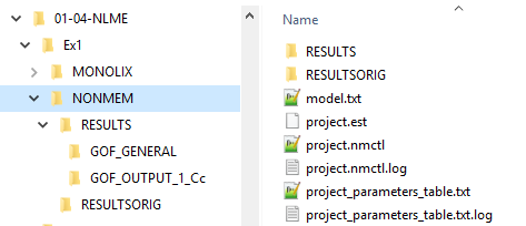
The RESULTSORIG folder contains the original NONMEM output. The ``RESULTS```folder contains by IQR Tools postprocessed output, such as diagnostic plots, and the convergence trajectories when the SAEM method is used. In the root of the project folder, in addition, a table with the parameter estimates is stored.
The structuring of an NLME project folder as shown above is identical for the MONOLIX model.
The reader is invited to browse the material him/herself to explore the output of the model runs.
In the following the different output elements for the model are shown, based on R command line commands, showing the same results as stored in the project folders.
11.1.6 Tabular results
In this example it is shown how the NLME project, generated in the previous example, can be processed with IQR Tools from command line to obtain information in the form of parameter tables.
As mentioned before, an IQRnlmeProject is identified by a relative path to the project folder. Such a path can be converted to an IQRnlmeProject object using the function as_IQRnlmeProject():
For IQRnlmeProject objects the generic print() and summary() functions are available.
The summary() functions generates a parameter estimates table with humanly understandable information.
This table is also stored in the project folder as project_parameters_table.txt file in a Word reporting ready format (using IQReport).
##    Population parameter estimates
##    =============================================================================================================
##
##    PARAMETER                        | VALUE  | RSE   | SHRINKAGE | COMMENT
##    -------------------------------------------------------------------------------------------------------------
##    **Typical parameters**           |        |       |           |
##    ka                               | 0.0854 | 5.88% | -         | (1/hour) Absorption rate
##    CL                               | 3.47   | 6.94% | -         | (L/hour) Apparent clearance
##    Vc                               | 2.14   | 25.3% | -         | (L) Apparent volume of distribution
##                                     |        |       |           |
##    **Inter-individual variability** |        |       |           |
##    omega(ka)                        | 0.0213 | 830%  | 88.2%     | LogNormal
##    omega(CL)                        | 0.183  | 44.1% | 0.6%      | LogNormal
##    omega(Vc)                        | 0.572  | 32.6% | 2.8%      | LogNormal
##                                     |        |       |           |
##    **Residual Variability**         |        |       |           |
##    error_ADD1                       | 0.751  | 5.31% | 10.1%*    | Additive Error (ug/ml) - Plasma concentration
##                                     |        |       |           |
##    Objective function               | 118    | -     | -         | -
##    AIC                              | 132    | -     | -         | -
##    BIC                              | 152    | -     | -         | -
##    -------------------------------------------------------------------------------------------------------------
## Model: material/01-04a-X1-NLME/Ex1/NONMEM/, Significant digits: 3 (Objective function rounded to closest integer value), omega values and error model parameters reported in standard deviation.
## As suggested in the NONMEM manual, the objective function was determined using importance sampling (IMP) with settings EONLY=1 and MAPITER=0.
## \* Epsilon shrinkage (records with missing dependent variable and censored records not considered).
##
## IQRoutputTable object
The print() function generates for NONMEM models information similar to obtained from MONOLIX directly as the summary.txt file. This information is also stored in the projects RESULTS folder as project_results.txt.
## ========================================================================================================
##     Summary results
##     Project: material/01-04a-X1-NLME/Ex1/NONMEM
## ========================================================================================================
##
## --------------------------------------------------------------------------------------------------------
## Termination information (Method(s): ITS,SAEM,IMP)
## --------------------------------------------------------------------------------------------------------
##     OPTIMIZATION WAS NOT TESTED FOR CONVERGENCE
##
##     STOCHASTIC PORTION WAS NOT TESTED FOR CONVERGENCE
##     REDUCED STOCHASTIC PORTION WAS COMPLETED
##
##     EXPECTATION ONLY PROCESS WAS NOT TESTED FOR CONVERGENCE
##
## --------------------------------------------------------------------------------------------------------
## Name                           Value          stderr         RSE (%)          95%CI
## --------------------------------------------------------------------------------------------------------
## log(ka)                       -2.461         0.05875           2.387
## log(CL)                        1.245         0.06938           5.572
## log(Vc)                       0.7608           0.253           33.26
##
## ka                           0.08535        0.005015           5.875
## CL                             3.473           0.241           6.938
## Vc                              2.14          0.5415            25.3
##
## omega(ka)                    0.02126          0.1765           830.3
## omega(CL)                     0.1828         0.08063            44.1
## omega(Vc)                     0.5721          0.1864           32.58
##
##
## error_ADD1                    0.7513         0.03993           5.315
##
## --------------------------------------------------------------------------------------------------------
## Correlation of fixed effects and covariate coefficients
## --------------------------------------------------------------------------------------------------------
## ka            1
## CL        0.068           1
## Vc        -0.14        0.18           1
##
## Eigenvalues (min, max, max/min): 0.73  1.20  1.64
##
## --------------------------------------------------------------------------------------------------------
## Correlation of random effects (variances) and error parameters
## --------------------------------------------------------------------------------------------------------
## omega2(ka)                   1
## omega2(CL)              -0.061           1
## omega2(Vc)               0.089       -0.22           1
## error_ADD1               0.022       0.096        0.41           1
##
## Eigenvalues (min, max, max/min): 0.49  1.45  2.98
##
## --------------------------------------------------------------------------------------------------------
## Objective function (IMP)
## --------------------------------------------------------------------------------------------------------
## OFV:    118.307
## AIC:    132.307
## BIC:    151.82
##
##
## IQRnlmeProject: material/01-04a-X1-NLME/Ex1/NONMEM/
In addition, functions are available to show tabular results for multiple NLME models. As a basis for handling multiple NLME models, the as_IQRnlmeProjectMulti() function is used. In the following example we generate such an IQRnlmeProjectMulti project for the NONMEM and MONOLIX model in the previous examples:
pM <- as_IQRnlmeProjectMulti(c(
  "material/01-04a-X1-NLME/Ex1/MONOLIX",
  "material/01-04a-X1-NLME/Ex1/NONMEM"))
names(pM) <- c("MONOLIX Model", "NONMEM Model")
The compareModels_IQRnlmeProject() function can be used to generate a table that compares the parameter estimates for the models contained in the IQRnlmeProjectMulti object. Using the filename argument in the compareModels_IQRnlmeProject() function, the same table can easily be exported to a file that then can be reported to MS Word with IQReport. Here we just display the table:
##    Comparison of model results for multiple models
##    ===============================================
##
##    Parameter  | MONOLIX Model | NONMEM Model
##    -----------------------------------------------
##    ka         | 0.0852 (6.1%) | 0.0854 (5.9%)
##    CL         | 3.46 (6.5%)   | 3.47 (6.9%)
##    Vc         | 2.12 (18%)    | 2.14 (25%)
##               |               |
##    omega(ka)  | 0.0912 (78%)  | 0.0213 (830%)
##    omega(CL)  | 0.185 (24%)   | 0.183 (44%)
##    omega(Vc)  | 0.564 (23%)   | 0.572 (33%)
##               |               |
##    error_ADD1 | 0.741 (7.5%)  | 0.751 (5.3%)
##               |               |
##    OBJ        | 339           | 118
##    BIC        | 356           | 152
##    AIC        | 353           | 132
##    -----------------------------------------------
## FIX (parameter fixed to this value), - (parameter not used)
## Number of significant digits: 3.
## Relative standard errors (RSE) given in parenthesis with 2 significant digits.
## Model metrics (OBJ, AIC, BIC) are rounded to nearest integer., MONOLIX Model (material/01-04a-X1-NLME/Ex1/MONOLIX), NONMEM Model (material/01-04a-X1-NLME/Ex1/NONMEM)
##
## IQRoutputTable object
Also for IQRnlmeProjectMulti objects a summary() function is available. A filename argument exists for this function, allowing to save results to disk.
The summary information contains a table with objective function information and the user provided comment:
##    Model overview table with model comments
##    =========================================================================================
##
##    MODEL         | OBJ | AIC | BIC | COMMENT
##    -----------------------------------------------------------------------------------------
##    MONOLIX Model | 339 | 353 | 356 | 1 cpt model with 1st order absorption - MONOLIX version
##    NONMEM Model  | 118 | 132 | 152 | 1 cpt model with 1st order absorption - NONMEM version
##    -----------------------------------------------------------------------------------------
## Objective function values (OBJ, AIC, BIC) are rounded.
##
## IQRoutputTable object
In addition it provides a table with information about fixed effect, random effect, and error model parameter estimates for each model.
##    Parameter estimates (fixed effects, error model, random effects) and their relative standard errors
##    ==========================================================================================================
##
##    MODEL                             | OBJ     | ka            | CL            | Vc            | error_ADD1
##    ----------------------------------------------------------------------------------------------------------
##    **Fixed effects / Errors (RSE%)** |         |               |               |               |
##    MONOLIX Model                     | 339     | 0.0852 (6.1%) | 3.46 (6.5%)   | 2.12 (18%)    | 0.741 (7.5%)
##    NONMEM Model                      | 118     | 0.0854 (5.9%) | 3.47 (6.9%)   | 2.14 (25%)    | 0.751 (5.3%)
##                                      |         |               |               |               |
##    **Random effects (RSE%)**         | **OBJ** | **omega(ka)** | **omega(CL)** | **omega(Vc)** |
##    MONOLIX Model                     | 339     | 0.0912 (78%)  | 0.185 (24%)   | 0.564 (23%)   |
##    NONMEM Model                      | 118     | 0.0213 (830%) | 0.183 (44%)   | 0.572 (33%)   |
##    ----------------------------------------------------------------------------------------------------------
## Number of significant digits: 3.
## Objective function values (OBJ, AIC, BIC) are rounded.
## Relative standard errors with 2 significant digits.
##
## IQRoutputTable object
Additional information about covariates and random effect correlations is generated by the summary() function but not further discussed here, as the model does not contain these features.
11.1.7 General diagnostics
Plotting diagnostic plots for an IQRnlmeProject can be done using the generic plot() function. The output argument of this function is a list of ggplot objects. After execution of run_IQRnlmeProject() all these plots are also available as PDF documents in the ``RESULTS```folder of the project.
You can view the generated PDFs here:
In this example we use an NLME model from the first example to generate plots from R command line:
Generate all plots
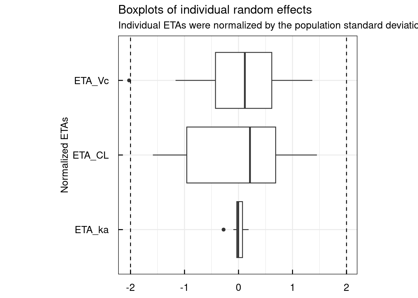
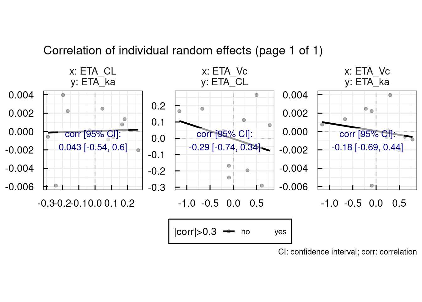
General diagnostic plots include:
# Random effect histograms compared to the estimated population variability
p$GENERAL$ETA$Histograms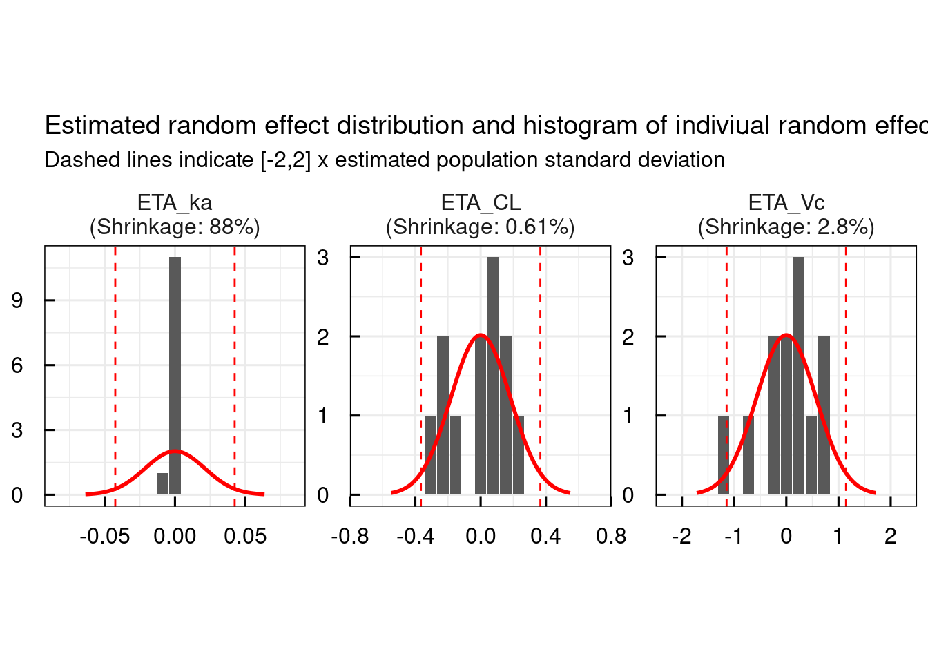
Convergence trajectories, in case SAEM was used, can be plotted using the following command. Also this plot is automatically generated and exported to PDF in the RESULTS folder of the project when running run_IQRnlmeProject().
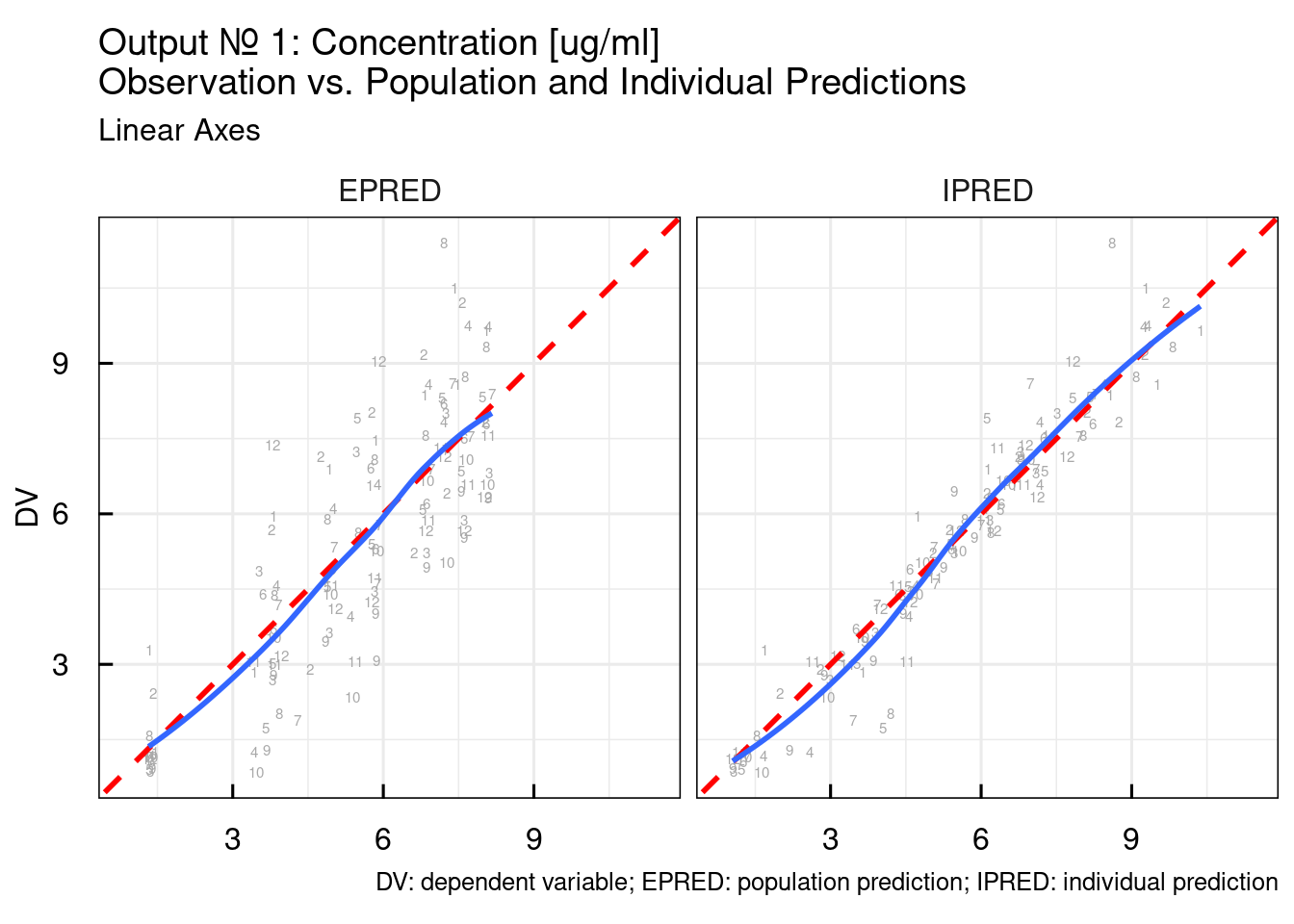
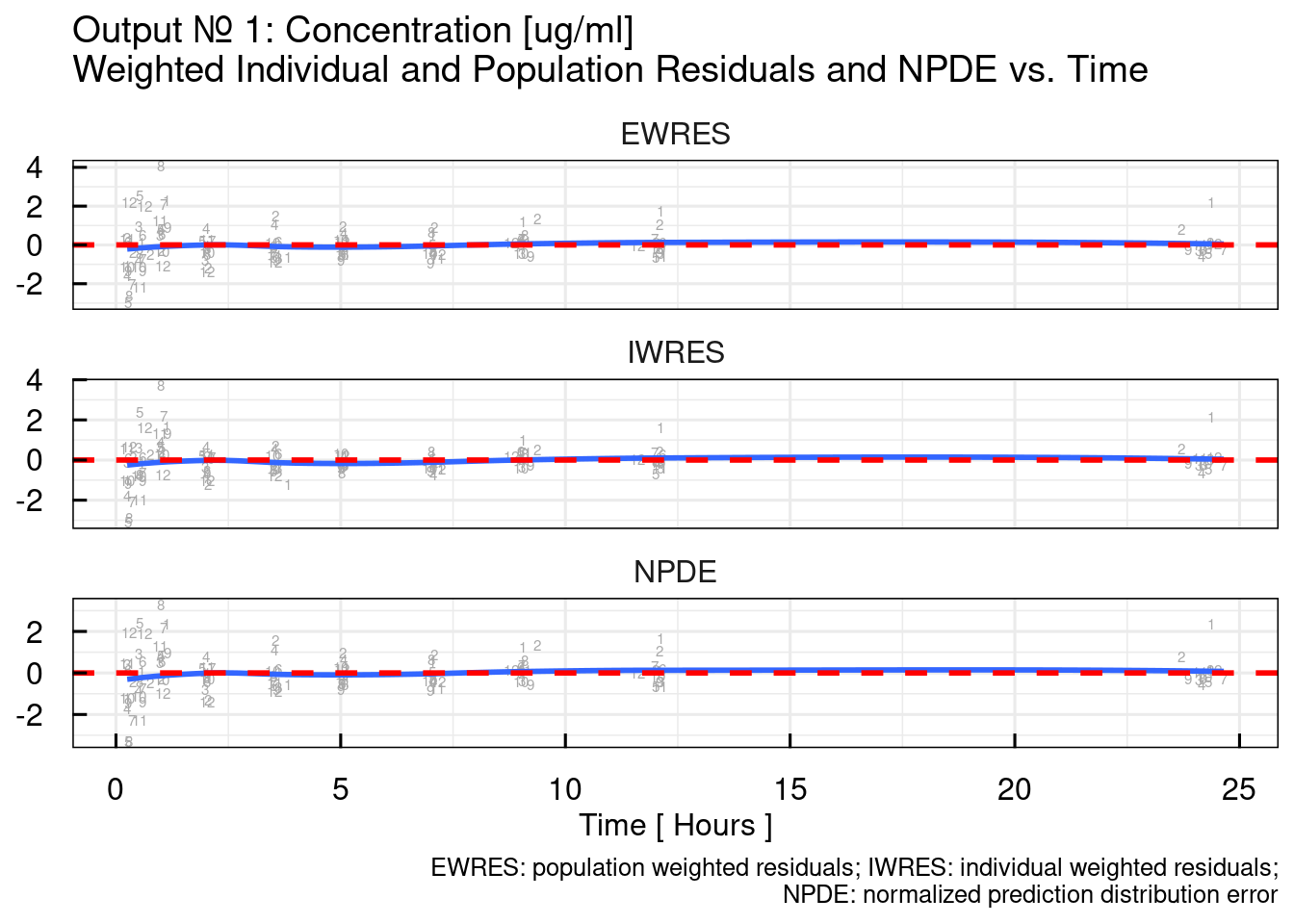
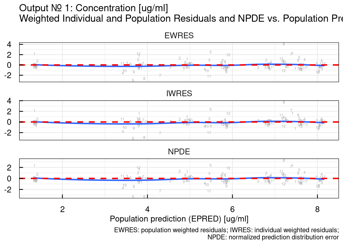
11.1.8 Output diagnostics
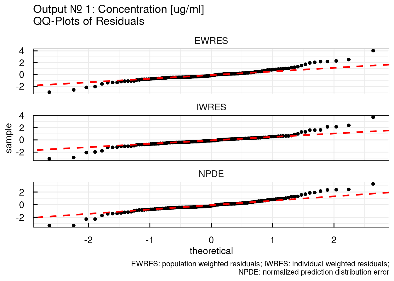
For each observed output in an NLME model, output specific diagnostic plots can be generated. All these plots are already generated during the execution of run_IQRnlmeProject() and stored as PDFs in the RESULTS folder.
You can view the generated PDFs here:
Here it is demonstrated how these results can be generated by command line … mainly for the purpose of showing the plots in a convenient manner. Normally, the PDFs are a good medium for assessment and also reporting. Instead of using the NONMEM model as in th previous example we will be using the MONOLIX example. IQR Tools is agnostic to the estimation tool and all functions will work the same, independently if NONMEM, MONOLIX, or NLMIXR was used for estimation.
Generate all plots
The output diagnostic plots include (for each output):
# Individual plots with data, individual and
# population predictions on a linear scale
p$OUTPUT$Cc$INDIVLIN[[1]]
# Individual plots with data, individual and
# population predictions on a log scale
p$OUTPUT$Cc$INDIVLOG[[1]]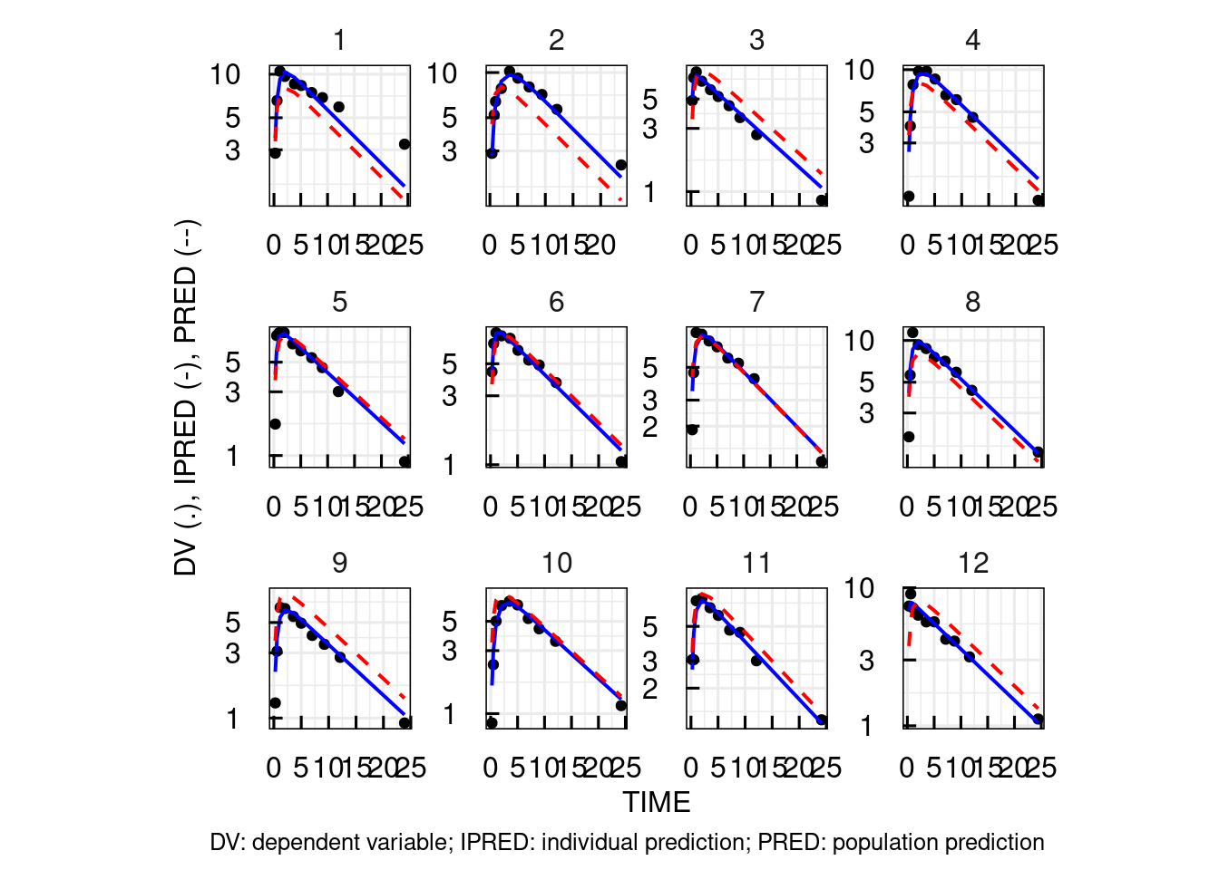
In the following not all plots but only selected are shown. For the full range of plots, please look in the book material in the respective project folders (material/01-04a-X1-NLME/Ex1/NONMEM/RESULTS).
11.1.9 Lagtime and FOCEI
In this example the model from Example 1 is used again but now we would like to estimate a lag time parameter on the dosing input. Additionally, we would like to use FOCEI instead of SAEM with NONMEM.
The data is defined as previously:
data          <- data_IQRest(
  datafile       = "material/01-04a-X1-NLME/Ex1/data.csv",  # absolute or relative path to the dataset
  covNames       = c("WT0"),      # specifying continuos candidate covariates
  catNames       = c("SEX")       # vector with names of categorical covariates
)
The structural model is defined as previously:
In the dosing object the name of the lag time parameters to be used is to be defined. Here we chose the default name of Tlag1:
In the model specification object, now in addition, also the initial guess for the Tlag1 parameter needs to be defined.
## Model specification
modelSpec     <- modelSpec_IQRest(
  # Defining the initial guesses for the fixed effect parameters
  # Here in addition to the first example also the guess for the lag time parameter
  POPvalues0  = c(CL=40, Vc=2, ka=2, Tlag1=0.5)
)
The estimation object is built as before:
## Building estimation object
est <- IQRnlmeEst(model         = model,
                  dosing        = dosing,
                  data          = data,
                  modelSpec     = modelSpec)
The projects are generated as before. The main difference here is that a different path (Ex5) was chosen and the comment was changed to include information about that lag time is tested in this model. In addition, the argument algOpt.NONMEM.METHOD was set to “FOCEI” and the importance sampling to generate the correct objective function after the main estimation run was switchd off by algOpt.NONMEM.IMPORTANCESAMPLING=FALSE.
# Creating a NONMEM project
projNONMEM <- IQRnlmeProject(est = est,
                             projectPath="material/01-04a-X1-NLME/Ex5/NONMEM",
                             tool="NONMEM",
                             algOpt.NONMEM.METHOD = "FOCEI",
                             algOpt.NONMEM.IMPORTANCESAMPLING = FALSE,
                             comment = "1 cpt model with 1st order absorption and lag time - NONMEM version")

# Creating a MONOLIX project
projMONOLIX <- IQRnlmeProject(est = est,
                              projectPath="material/01-04a-X1-NLME/Ex5/MONOLIX",
                              tool="MONOLIX",
                              algOpt.K1 = 50,
                              algOpt.K2 = 20,
                              comment = "1 cpt model with 1st order absorption and lag time  - MONOLIX version")
In this documentation these models are not executed.
The generated control files can be found here:
11.1.10 Zero-order absorption
In this example the model from Example 1 is used again but now we would like to implement a sequential 0th- and 1st-order absorption with lagtime.
The data is defined as previously:
data          <- data_IQRest(
  datafile       = "material/01-04a-X1-NLME/Ex1/data.csv",  # absolute or relative path to the dataset
  covNames       = c("WT0"),      # specifying continuos candidate covariates
  catNames       = c("SEX")       # vector with names of categorical covariates
)
The structural model is defined similarly as before. However, there is one difference: the parameter that is going to be used to represent the value of the zero-order absorption time to be estimated needs to be defined in the structural model as parameter. Here the parameter name Tk0 is chosen and in the structural model it is initialized with an arbitrary value of 0. The structural model can be seen here.
In the dosing object the name of the zero-order absorption parameter needs to be defined in addition to the lag time parameter, using the Tk0 argument:
In the model specification object, now in addition, also the initial guesses for the Tlag1 and Tk0 parameters need to be defined.
## Model specification
modelSpec     <- modelSpec_IQRest(
  # Defining the initial guesses for the fixed effect parameters
  # Here in addition to the first example also the guess for the
  # lag time and 0 order absorption time parameters need to be defined
  POPvalues0  = c(CL=40, Vc=2, ka=2, Tlag1=0.5, Tk0=0.5)
)
The estimation object is built as before:
## Building estimation object
est <- IQRnlmeEst(model         = model,
                  dosing        = dosing,
                  data          = data,
                  modelSpec     = modelSpec)
The projects are generated as before. The main difference here is that a different path (Ex6) was chosen and the comment was changed to include information about that lag time and 0 order absorption is tested in this model.
# Creating a NONMEM project
projNONMEM <- IQRnlmeProject(est = est,
                             projectPath="material/01-04a-X1-NLME/Ex6/NONMEM",
                             tool="NONMEM",
                             algOpt.NONMEM.METHOD = "FOCEI",
                             algOpt.NONMEM.IMPORTANCESAMPLING = FALSE,
                             comment = "1 cpt model with 0th/1st order absorption and lag time - NONMEM version")

# Creating a MONOLIX project
projMONOLIX <- IQRnlmeProject(est = est,
                              projectPath="material/01-04a-X1-NLME/Ex6/MONOLIX",
                              tool="MONOLIX",
                              algOpt.K1 = 50,
                              algOpt.K2 = 20,
                              comment = "1 cpt model with 0th/1st order absorption and lag time  - MONOLIX version")
In this documentation these models are not executed.
The generated control files can be found here:
11.1.11 NLME model settings
In the previous examples only initial guesses for parameters were provided for the model specification and all other settings were left on default values. In this example additional model specification arguments are introduced. Specifically, we consider the following model settings:
- Use of regression parameters (individual PK parameters provided in the dataset)
- Fix or estimate a fixed effect
- Set initial guesses for random effects
- Fix, estimate, or remove a random effect
- Normal, lognormal, or logitnormal distribution of individual parameters
- Additive, proportional, or additive proportional error model
The underlying structural model for this example is two-compartmental linear PK model with IV input and a PD model based on Friberg et al. 2002.
A matching simulated dataset is provided that contains measurements for neutrophil levels, corresponding to the output in the model. The individual PK parameters are provided as columns in the dataset.
| IXGDF | USUBJID | ID | TIME | TIMEPOS | TAD | NAME | DV | UNIT | YTYPE | AMT | ADM | EVID | MDV | CENS | TINF | RATE | Vp | Vc | CL | Q | WT | HT |
|---|---|---|---|---|---|---|---|---|---|---|---|---|---|---|---|---|---|---|---|---|---|---|
| 1 | 1 | 1 | 0 | 0 | 0 | Dose | 0.0 | mg | 0 | 206 | 1 | 1 | 1 | 0 | 0.5 | 412 | 454 | 272 | 236 | 102 | 84 | 183 |
| 2 | 1 | 1 | 0 | 0 | 0 | Neutrophils | 8.1 | 10^9/L | 1 | 0 | 0 | 0 | 0 | 0 | 0.0 | 0 | 454 | 272 | 236 | 102 | 84 | 183 |
| 3 | 1 | 1 | 192 | 192 | 192 | Neutrophils | 3.3 | 10^9/L | 1 | 0 | 0 | 0 | 0 | 0 | 0.0 | 0 | 454 | 272 | 236 | 102 | 84 | 183 |
| 4 | 1 | 1 | 336 | 336 | 336 | Neutrophils | 5.5 | 10^9/L | 1 | 0 | 0 | 0 | 0 | 0 | 0.0 | 0 | 454 | 272 | 236 | 102 | 84 | 183 |
| 5 | 1 | 1 | 456 | 456 | 456 | Neutrophils | 12.3 | 10^9/L | 1 | 0 | 0 | 0 | 0 | 0 | 0.0 | 0 | 454 | 272 | 236 | 102 | 84 | 183 |
| 6 | 2 | 2 | 0 | 0 | 0 | Dose | 0.0 | mg | 0 | 165 | 1 | 1 | 1 | 0 | 0.5 | 330 | 471 | 153 | 202 | 102 | 84 | 167 |
| 7 | 2 | 2 | 0 | 0 | 0 | Neutrophils | 11.9 | 10^9/L | 1 | 0 | 0 | 0 | 0 | 0 | 0.0 | 0 | 471 | 153 | 202 | 102 | 84 | 167 |
| 8 | 2 | 2 | 432 | 432 | 432 | Neutrophils | 9.7 | 10^9/L | 1 | 0 | 0 | 0 | 0 | 0 | 0.0 | 0 | 471 | 153 | 202 | 102 | 84 | 167 |
| 9 | 3 | 3 | 0 | 0 | 0 | Dose | 0.0 | mg | 0 | 172 | 1 | 1 | 1 | 0 | 0.5 | 344 | 635 | 250 | 222 | 102 | 78 | 175 |
| 10 | 3 | 3 | 0 | 0 | 0 | Neutrophils | 6.4 | 10^9/L | 1 | 0 | 0 | 0 | 0 | 0 | 0.0 | 0 | 635 | 250 | 222 | 102 | 78 | 175 |
Please consider the code piece below. It explains the different features, mentioned above in the inline documentation.
Specifically have a look at the arguments POPestimate, IIVvalues0, IIVestimate, IIVdistribution, and errorModel of the modelSpec_IQRest() function.
# Load the structural model
model         <- IQRmodel("material/01-04a-X1-NLME/Ex7/model.txt")

# Define type of dosing
dosing        <- dosing_IQRest(
  INPUT1 = c(type="INFUSION")
)

# Define data information
data          <- data_IQRest(
  datafile       = "material/01-04a-X1-NLME/Ex7/data.csv",
  # The covariates height (HT) and weight (WT) are available in the dataset
  covNames       = c("WT","HT"),

  # The individual PK parameters CL, Vc, Q, and Vp are defined in the dataset
  # The names of these columns need to be defined here - in the order of appearance in
  # the dataset.
  regressorNames = c("CL","Vc","Q","Vp")
)

# Define model specifications related to the parameter, statistical, covariate model
modelSpec     <- modelSpec_IQRest(

  # The only required argument is POPvalues0 which codes for the initial guesses of the parameters
  POPvalues0      = c(CIRC0=7.21, MTT=124, SLOPU=28.9, GAM=0.239),

  # The POPestimate argument is a named vector that needs to contain the same elements as
  # POPvalues0. Values can be 0 or 1 with the folowing meaning
  #   0: the parameter is not estimated but kept fixed on the initial guess
  #   1: the fixed effect parameter is estimated (default if POPestimate not defined)
  # Here: the GAM coefficient is not estimated but kept fixed on a value of 0.239.
  POPestimate     = c(CIRC0=1,    MTT=1,   SLOPU=1,    GAM=0),

  # The IIVvalues0 argument is a named vector that needs to contain the same elements as
  # POPvalues0. The values define the initial guesses for the random effect on the respective
  # parameter. The values represent standard deviations! If IIVvalues0 is not defined, default
  # values of 0.5 are used.
  IIVvalues0     = c(CIRC0=0.2,   MTT=0.4, SLOPU=0.3,  GAM=0),

  # The IIVestimate argument is a named vector that needs to contain the same elements as
  # POPvalues0. Values can be 0, 1, or 2 with the folowing meaning
  #   0: no random effect is used (fixed to 0, independently of value defined in IIVvalues0
  #   1: the random effect parameter is estimated (default if IIVestimate not defined)
  #   2: the random effect parameter is kept fixed on its initial guess
  # Here: There is no random effect on the GAM coefficient. The random effect for the
  # drug effect parameter SLOPU is fixed to 0.3. All other random effects are estimated.
  IIVestimate     = c(CIRC0=1,    MTT=1,   SLOPU=2,    GAM=0),

  # The IIVdistribution argument is a named vector that needs to contain the same elements as
  # POPvalues0. Values can be "N", "L", or "G"" with the folowing meaning
  #   "N": Individual parameters assumed normally distributed (can be 0, positive, and negative)
  #   "L": Individual parameters assumed lognormally distributed (>0) (default if IIVdistribution not defined)
  #   "G": Individual parameters assumed logitnormally distributed (values between 0 and 1)
  # Here: the GAM coefficient is assumed to be normally distributed.
  # All other parameters assumed lognormally distributed.
  IIVdistribution = c(CIRC0="L",  MTT="L", SLOPU="L",  GAM="N"),

  # The model contains one observed output. The argument "errorModel" allows to define the
  # type of residual error model. If errorModel argument is not present, the default error
  # models ar additive error models for all outputs. If errorModel argument is defined then
  # it has to be defined for all outputs as a named list. The names are the names of the
  # outputs (OUTPUT1, OUTPUT2, etc.). In the example below, a proportional error
  # model is chosen for the neutrophils. An initial guess for the error parameter is
  # defined.
  # Examples for coding additive proportional and additive error models are below:
  #
  # OUTPUT1 = c("absrel", 1, 0.3) # Additive proportional error model with 1 as guess
  #                                 for additiv, and 0.3 for proportional part
  # OUTPUT1 = c("abs", 1) # Additive error model with 1 as guess for additiv part

  errorModel = list(
    OUTPUT1 = c("rel", 0.3)
  )
)

# Create IQRnlmeEst object
est <- IQRnlmeEst(model         = model,
                  dosing        = dosing,
                  data          = data,
                  modelSpec     = modelSpec)
Projects can be generated with the IQRnlmeProject() function, as discussed in previous examples:
# Creating a NONMEM project
projNONMEM <- IQRnlmeProject(est = est,
                             projectPath="material/01-04a-X1-NLME/Ex7/NONMEM",
                             tool="NONMEM",
                             algOpt.K1 = 50,
                             algOpt.K2 = 20,
                             algOpt.NONMEM.ITS = FALSE,
                             algOpt.NONMEM.IMPORTANCESAMPLING = FALSE,
                             comment = "PKPD model - NONMEM version")

# Creating a MONOLIX project
projMONOLIX <- IQRnlmeProject(est = est,
                              projectPath="material/01-04a-X1-NLME/Ex7/MONOLIX",
                              tool="MONOLIX",
                              algOpt.K1 = 50,
                              algOpt.K2 = 20,
                              comment = "PKPD model - MONOLIX version")
The projects are run. In this case the optional argument ncores is defined, allowing to set the number of cores on which to execute the NONMEM and / or MONOLIX model. Note that for parallel execution the NONMEM installation needs to be appropriate.
# Run the NONMEM model
run_IQRnlmeProject("material/01-04a-X1-NLME/Ex7/NONMEM",ncores = 4)

# Run the MONOLIX model
run_IQRnlmeProject("material/01-04a-X1-NLME/Ex7/MONOLIX",ncores = 8)
The generated control files can be found here:
The reader is invited to have a look at the book example material at the output of the model runs.
11.1.12 Sequential PK/PD
Sequential PK/PD modeling means that a PK model was executed to obtain the individual PK parameters. These then are added to the PD modeling dataset and accessed from the PD model to inform the PK parameters. Only the PD parameters then are estimated.
An example for how available PK parameters can be used in a subsequent PD model fit is available in the NLME model settings example.
11.1.13 Regression parameters
Regression parameters are model parameters whos values are passed to the model upon estimation via the dataset. These can be time dependent or independent. Their use can be sequential model building but these parameters can also be used to implement complex covariate models. Please refer to the hyperlinked sections to learn more.
11.1.14 Error models
Error models for observables in NLME models are defined using the argument errorModel in the function modelSpec_IQRest(). One error model per observable / model output needs to be defined. If the errorModel argument is missing, an additive error model will be used for each outputs.
The errorModel argument is a named list. The names of the elements need to have the same names as the output identifiers in the structural model (OUTPUT1, OUTPUT2, OUTPUT3, etc.). The values are vectors. The first entry is either abs for an additive error model, rel for a proportional error model, or absrel for an additive-proportional error model. The following entries in the vector code for the initial guesses of the error model parameters. In case of an additive-proportional error model the additive error parameter guess is defined first, followed by the proportional error parameter.
Exponential or more complex error models are not implemented in an automatic manner. In case of exponential error models, this can be implemented by log transforming of the data. Bounded error models can also be implemented by suitable transformations of the observed data.
An example for an error model definition for three outputs is shown below:
11.1.15 Multiple outputs
Multiple outputs typically occur in parent/metabolite PK models. But can also be found in case of joint PK/PD models.
In this case the observations for several outputs are coded in the dataset. The structural model requires the presence of multiple output definition (OUTPUT1, OUTPUT2, …). When setting up the NLME model specification using the function modelSpec_IQRest() the only thing which needs to be one in addition is to define an error model for each output.
Assuming there are 3 observables, the errorModel argument in the modelSpec_IQRest() function could be defined as follows, containing one error model definition per output/observable:
For more information about the definition of error models, see this section.
11.1.16 Basic covariate models
In this section the basic covariate model implementation is documented. A simulated PK NLME modeling dataset with the baseline covariates weight (WT0), age (AGE0), height (HT0), BMI (BMI0), and gender (SEX) is provided.
| ID | TIME | TIMEUNIT | YTYPE | NAME | DV | UNIT | MDV | EVID | AMT | ADM | TINF | RATE | DOSE | WT0 | AGE0 | BMI0 | HT0 | SEX |
|---|---|---|---|---|---|---|---|---|---|---|---|---|---|---|---|---|---|---|
| 3 | 0.000 | HOURS | NA | Dose | 0.00 | ug | 1 | 1 | 1000 | 1 | 0 | 0 | 1000 | 80 | 28 | 24.69 | 180 | 1 |
| 3 | 0.250 | HOURS | 1 | Concentration | 1.53 | ng/ml | 0 | 0 | 0 | NA | 0 | 0 | 1000 | 80 | 28 | 24.69 | 180 | 1 |
| 3 | 0.500 | HOURS | 1 | Concentration | 3.50 | ng/ml | 0 | 0 | 0 | NA | 0 | 0 | 1000 | 80 | 28 | 24.69 | 180 | 1 |
| 3 | 1.000 | HOURS | 1 | Concentration | 3.80 | ng/ml | 0 | 0 | 0 | NA | 0 | 0 | 1000 | 80 | 28 | 24.69 | 180 | 1 |
| 3 | 2.000 | HOURS | 1 | Concentration | 3.33 | ng/ml | 0 | 0 | 0 | NA | 0 | 0 | 1000 | 80 | 28 | 24.69 | 180 | 1 |
| 3 | 4.000 | HOURS | 1 | Concentration | 2.91 | ng/ml | 0 | 0 | 0 | NA | 0 | 0 | 1000 | 80 | 28 | 24.69 | 180 | 1 |
| 4 | 0.000 | HOURS | NA | Dose | 0.00 | ug | 1 | 1 | 1000 | 1 | 0 | 0 | 1000 | 68 | 25 | 24.68 | 166 | 1 |
| 4 | 0.083 | HOURS | 1 | Concentration | 1.38 | ng/ml | 0 | 0 | 0 | NA | 0 | 0 | 1000 | 68 | 25 | 24.68 | 166 | 1 |
| 4 | 0.250 | HOURS | 1 | Concentration | 2.12 | ng/ml | 0 | 0 | 0 | NA | 0 | 0 | 1000 | 68 | 25 | 24.68 | 166 | 1 |
| 4 | 0.500 | HOURS | 1 | Concentration | 3.59 | ng/ml | 0 | 0 | 0 | NA | 0 | 0 | 1000 | 68 | 25 | 24.68 | 166 | 1 |
A linear 2 compartment distribution model with first-order absorption is provided as structural model.
In the following the following is demonstrated:
- Selection of covariates to be used on parameters
- Setting initial guesses for covariate coefficients
- Fixing covariate coefficients to values
- Centering covariates
11.1.16.1 Basic covariate model with estimated coefficients
A basic covariate model can be defined by defining the covariateModel argument of modelSpec_IQRest(), linking covariates to be used to parameters. The following example shows how to add the covariate SEX on ka, WT0 on CL, and AGE0 on CL and Vc. See the inline documentation for more information.
# Structural model
model <- IQRmodel("material/01-04a-X1-NLME/Ex8/model.txt")

# Data definition
data <- data_IQRest(
  datafile = "material/01-04a-X1-NLME/Ex8/data.csv",
  covNames = c("HT0", "WT0", "AGE0","BMI0"),
  catNames = "SEX"
)

# Dosing definition
dosing <- dosing_IQRest(
  INPUT1 = c(type = "BOLUS")
)

# Model specification
modelSpec <- modelSpec_IQRest(

  # Typical subject parameters
  POPvalues0  = c(ka = 0.2, CL = 20, Vc = 20, Q1 = 20, Vp1 = 2000),

  # Estimation settings for fixed effect parameters
  POPestimate = c(ka = 1  , CL =  1, Vc =  1, Q1 =  1, Vp1 =    1),

  # Inter-individual variability settings
  IIVdistribution = c(ka ="L" , CL ="L" , Vc ="L" , Q1 ="L" , Vp1 ="L"  ),
  IIVvalues0      = c(ka = 0.5, CL = 0.5, Vc = 0.5, Q1 = 0.5, Vp1 = 0.1 ),
  IIVestimate     = c(ka = 1  , CL = 1  , Vc = 1  , Q1 = 1  , Vp1 = 1   ),

  # Definition of the covariate model.
  # The covariateModel argument is a named list. The names of the elements need
  # to be parameters in the model on which to add a covariate. The values are
  # character strings that contain the names of the covariates to add to the parameter.
  #
  # Default settings:
  # 1) Continuous covariates are centered around the median of the covariate in the population
  #    and log transformed: log(cov/median). For lognormally transformed parameters this results
  #    in the exponential covariate model: PARAM = TPARAM*(cov/median)^beta, where beta is the estimated
  #    covariate coefficient. For normally transformed parameters this results in PARAM = TPARAM + beta*log(cov/median).
  # 2) The reference category for categorical covariates is the category with the smallest value.
  #    In the MU domain categorial covariates are implemented by:
  #    trans(PARAM) = trans(TPARAM) + beta*(cat==category)
  #    where trans is the transformation, beta the covariate coefficient,and (cat==category) is 1 if the categorical
  #    covariate is equal to the tested covariate and 0 otherwise. For normally transformed parameters
  #    this results in: PARAM = TPARAM + beta*(cat==category)
  #    For lognormally transformed parameters in: PARAM = TPARAM*exp(beta*(cat==category))
  covariateModel = list(
    ka = c("SEX"),
    CL = c("WT0","AGE0"),
    Vc = c("AGE0")
  ),

  # Error model
  errorModel = list(
    OUTPUT1 = c(type="absrel",guess=c(1,0.3))
  )
)

# Create IQRnlmeEst object
est <- IQRnlmeEst(model         = model,
                  dosing        = dosing,
                  data          = data,
                  modelSpec     = modelSpec)
# Creating a NONMEM project
projNONMEM <- IQRnlmeProject(est = est,
projectPath="material/01-04a-X1-NLME/Ex8/NONMEM1",
tool="NONMEM",
algOpt.K1 = 100,
algOpt.K2 = 50,
algOpt.NONMEM.ITS = FALSE,
algOpt.NONMEM.IMPORTANCESAMPLING = FALSE,
comment = "First covariate model")
# Creating a MONOLIX project
projMONOLIX <- IQRnlmeProject(est = est,
projectPath="material/01-04a-X1-NLME/Ex8/MONOLIX1",
tool="MONOLIX",
algOpt.K1 = 50,
algOpt.K2 = 20,
comment = "First covariate model") In this documentation only the NONMEM model is executed.
The generated control files can be found here:
11.1.16.2 Implementation of basic covariates with IQR Tools
Continuous covariates are centered and log transformed log(cov/center). If not otherwise specified, the value for centering is the median value in the population. IQR Tools allows to set custom centering values, as will be shown in the next examples.
For lognormally transformed parameters this results in the exponential covariate model:
PARAM = TPARAM*(cov/center)^beta
where beta is the estimated covariate coefficient.
For normally transformed parameters this results in
PARAM = TPARAM + beta*log(cov/center)
The reference category for categorical covariates is by default the category with the smallest value. However, IQR Tools also allows to freely choose the reference category among the available categories of a categorical covariate. This will be shown in the next examples.
In the MU domain categorial covariates are implemented by:
trans(PARAM) = trans(TPARAM) + beta*(cat==category)
where trans() is the transformation, beta the covariate coefficient,and (cat==category) is 1 if the categorical covariate is equal to the tested covariate and 0 otherwise. For normally transformed parameters this results in:
PARAM = TPARAM + beta*(cat==category)
For lognormally transformed parameters in:
PARAM = TPARAMexp(beta(cat==category))
For most analyses this implementation of covariates is sufficient. However, in certain cases more freedom is required. The implementation of fully customizable covariate models is discussed in section Complexe covariate models.
11.1.16.3 Centering of covariates
In the following example the centering of continuous covariates and the choice of the reference categories for categorical covariates is demonstrated. See the inline documentation of the code.
# Structural model
model <- IQRmodel("material/01-04a-X1-NLME/Ex8/model.txt")

# Data definition
data <- data_IQRest(
  datafile = "material/01-04a-X1-NLME/Ex8/data.csv",
  covNames = c("HT0", "WT0", "AGE0","BMI0"),
  catNames = "SEX"
)

# Dosing definition
dosing <- dosing_IQRest(
  INPUT1 = c(type = "BOLUS")
)

# Model specification
modelSpec <- modelSpec_IQRest(

  # Typical subject parameters
  POPvalues0  = c(ka = 0.2, CL = 20, Vc = 20, Q1 = 20, Vp1 = 2000),

  # Estimation settings for fixed effect parameters
  POPestimate = c(ka = 1  , CL =  1, Vc =  1, Q1 =  1, Vp1 =    1),

  # Inter-individual variability settings
  IIVdistribution = c(ka ="L" , CL ="L" , Vc ="L" , Q1 ="L" , Vp1 ="L"  ),
  IIVvalues0      = c(ka = 0.5, CL = 0.5, Vc = 0.5, Q1 = 0.5, Vp1 = 0.1 ),
  IIVestimate     = c(ka = 1  , CL = 1  , Vc = 1  , Q1 = 1  , Vp1 = 1   ),

  # Definition of the covariate model.
  covariateModel = list(
    ka = c("SEX"),
    CL = c("WT0","AGE0"),
    Vc = c("AGE0")
  ),

  # Centering of covariates can be done by definition of the COVcentering argument.
  # The value of this argument is a named vector. Then names correspond to the covariate names
  # and the values to the centering values (continuous) or reference categories (categorical).
  # Below a weight of 50kg was chosen as the centering for bodyweight and SEX=2 was chosen as
  # the reference category for SEX.
  COVcentering = c(WT0=50,SEX=2),

  # Error model
  errorModel = list(
    OUTPUT1 = c(type="absrel",guess=c(1,0.3))
  )
)

# Create IQRnlmeEst object
est <- IQRnlmeEst(model         = model,
                  dosing        = dosing,
                  data          = data,
                  modelSpec     = modelSpec)
Generate the projects:
# Creating a NONMEM project
projNONMEM <- IQRnlmeProject(est = est,
                             projectPath="material/01-04a-X1-NLME/Ex8/NONMEM2",
                             tool="NONMEM",
                             algOpt.K1 = 100,
                             algOpt.K2 = 50,
                             algOpt.NONMEM.ITS = FALSE,
                             algOpt.NONMEM.IMPORTANCESAMPLING = FALSE,
                             comment = "Second covariate model")

# Creating a MONOLIX project
projMONOLIX <- IQRnlmeProject(est = est,
                              projectPath="material/01-04a-X1-NLME/Ex8/MONOLIX2",
                              tool="MONOLIX",
                              algOpt.K1 = 50,
                              algOpt.K2 = 20,
                              comment = "Second covariate model")
The generated control files can be found here:
11.1.16.4 Covariate coefficient values
The example demonstrates how initial guesses for covariate coefficients can be provided. See the inline documentation of the code.
# Structural model
model <- IQRmodel("material/01-04a-X1-NLME/Ex8/model.txt")

# Data definition
data <- data_IQRest(
  datafile = "material/01-04a-X1-NLME/Ex8/data.csv",
  covNames = c("HT0", "WT0", "AGE0","BMI0"),
  catNames = "SEX"
)

# Dosing definition
dosing <- dosing_IQRest(
  INPUT1 = c(type = "BOLUS")
)

# Model specification
modelSpec <- modelSpec_IQRest(

  # Typical subject parameters
  POPvalues0  = c(ka = 0.2, CL = 20, Vc = 20, Q1 = 20, Vp1 = 2000),

  # Estimation settings for fixed effect parameters
  POPestimate = c(ka = 1  , CL =  1, Vc =  1, Q1 =  1, Vp1 =    1),

  # Inter-individual variability settings
  IIVdistribution = c(ka ="L" , CL ="L" , Vc ="L" , Q1 ="L" , Vp1 ="L"  ),
  IIVvalues0      = c(ka = 0.5, CL = 0.5, Vc = 0.5, Q1 = 0.5, Vp1 = 0.1 ),
  IIVestimate     = c(ka = 1  , CL = 1  , Vc = 1  , Q1 = 1  , Vp1 = 1   ),

  # Definition of the covariate model.
  covariateModel = list(
    ka = c("SEX"),
    CL = c("WT0","AGE0"),
    Vc = c("AGE0")
  ),

  # Centering of covariates
  COVcentering = c(WT0=50,SEX=2),

  # Initial guesses for covariate coefficients are provided as a list and assigned to the
  # argument covariateModelValues. The structure of this list is the same as the list for covariateModel.
  # The values are named vectors. If categorical covariates have multiple categories, the same guess is used.
  covariateModelValues = list(
    ka = c(SEX=0.4),
    CL = c(WT0=0.3,AGE0=0.6),
    Vc = c(AGE0=1)
  ),

  # Error model
  errorModel = list(
    OUTPUT1 = c(type="absrel",guess=c(1,0.3))
  )
)

# Create IQRnlmeEst object
est <- IQRnlmeEst(model         = model,
                  dosing        = dosing,
                  data          = data,
                  modelSpec     = modelSpec)
Generate the projects:
# Creating a NONMEM project
projNONMEM <- IQRnlmeProject(est = est,
                             projectPath="material/01-04a-X1-NLME/Ex8/NONMEM3",
                             tool="NONMEM",
                             algOpt.K1 = 100,
                             algOpt.K2 = 50,
                             algOpt.NONMEM.ITS = FALSE,
                             algOpt.NONMEM.IMPORTANCESAMPLING = FALSE,
                             comment = "Third covariate model")

# Creating a MONOLIX project
projMONOLIX <- IQRnlmeProject(est = est,
                              projectPath="material/01-04a-X1-NLME/Ex8/MONOLIX3",
                              tool="MONOLIX",
                              algOpt.K1 = 50,
                              algOpt.K2 = 20,
                              comment = "Third covariate model")
The generated control files can be found here:
11.1.16.5 Fixing covariate coefficients
The example demonstrates how covariate coefficients can be fixed. See the inline documentation of the code.
# Structural model
model <- IQRmodel("material/01-04a-X1-NLME/Ex8/model.txt")

# Data definition
data <- data_IQRest(
  datafile = "material/01-04a-X1-NLME/Ex8/data.csv",
  covNames = c("HT0", "WT0", "AGE0","BMI0"),
  catNames = "SEX"
)

# Dosing definition
dosing <- dosing_IQRest(
  INPUT1 = c(type = "BOLUS")
)

# Model specification
modelSpec <- modelSpec_IQRest(

  # Typical subject parameters
  POPvalues0  = c(ka = 0.2, CL = 20, Vc = 20, Q1 = 20, Vp1 = 2000),

  # Estimation settings for fixed effect parameters
  POPestimate = c(ka = 1  , CL =  1, Vc =  1, Q1 =  1, Vp1 =    1),

  # Inter-individual variability settings
  IIVdistribution = c(ka ="L" , CL ="L" , Vc ="L" , Q1 ="L" , Vp1 ="L"  ),
  IIVvalues0      = c(ka = 0.5, CL = 0.5, Vc = 0.5, Q1 = 0.5, Vp1 = 0.1 ),
  IIVestimate     = c(ka = 1  , CL = 1  , Vc = 1  , Q1 = 1  , Vp1 = 1   ),

  # Definition of the covariate model.
  covariateModel = list(
    ka = c("SEX"),
    CL = c("WT0","AGE0"),
    Vc = c("AGE0")
  ),

  # Centering of covariates
  COVcentering = c(WT0=50,SEX=2),

  # Initial guesses for covariate coefficients
  covariateModelValues = list(
    ka = c(SEX=0.4),
    CL = c(WT0=0.3,AGE0=0.6),
    Vc = c(AGE0=1)
  ),

  # Information about which covariate coefficients are estimated or not is provided as a list and
  # assigned to the argument COVestimate. The structure of this list is the same as the list for covariateModel.
  # The values are named vectors. A value of 0 means the covariate coefficient is not estimated but
  # kept fixed on the initial guess. A value of 1 mean it is estimated. If categorical covariates have
  # multiple categories, the same estimation setting is used for all categories.
  COVestimate = list(
    ka = c(SEX=1),
    CL = c(WT0=0,AGE0=1),
    Vc = c(AGE0=0)
  ),

  # Error model
  errorModel = list(
    OUTPUT1 = c(type="absrel",guess=c(1,0.3))
  )
)

# Create IQRnlmeEst object
est <- IQRnlmeEst(model         = model,
                  dosing        = dosing,
                  data          = data,
                  modelSpec     = modelSpec)
Generate the projects:
# Creating a NONMEM project
projNONMEM <- IQRnlmeProject(est = est,
                             projectPath="material/01-04a-X1-NLME/Ex8/NONMEM4",
                             tool="NONMEM",
                             algOpt.K1 = 100,
                             algOpt.K2 = 50,
                             algOpt.NONMEM.ITS = FALSE,
                             algOpt.NONMEM.IMPORTANCESAMPLING = FALSE,
                             comment = "Fourth covariate model")

# Creating a MONOLIX project
projMONOLIX <- IQRnlmeProject(est = est,
                              projectPath="material/01-04a-X1-NLME/Ex8/MONOLIX4",
                              tool="MONOLIX",
                              algOpt.K1 = 50,
                              algOpt.K2 = 20,
                              comment = "Fourth covariate model")
The generated control files can be found here:
11.1.17 Covariate plots
In the case that an NLME model contains covariate effects on parameters, additional diagnostics are generated when executing run_IQRnlmeProject(). These diagnostics are demonstrated here. As example NLME project we use the following:
project <- as_IQRnlmeProject("material/01-04a-X1-NLME/Ex8/NONMEM1")

# Create a summary table to see the contents
summary(project)
## Population parameter estimates
## ===========================================================================================================================
##
## PARAMETER | VALUE | RSE | SHRINKAGE | COMMENT
## ---------------------------------------------------------------------------------------------------------------------------
## **Typical parameters** | | | |
## ka | 0.207 | 6.33% | - | Absorption rate parameter (1/hour)
## CL | 32 | 9.22% | - | Apparent clearance (L/hour)
## Vc | 29.2 | 6.19% | - | Apparent central volume (L)
## Q1 | 22.6 | 4.92% | - | Apparent intercompartmental clearance (L/hour)
## Vp1 | 2260 | 4.94% | - | Apparent peripheral volume (L)
## | | | |
## **Inter-individual variability** | | | |
## omega(ka) | 0.336 | 9.02% | 6.4% | LogNormal
## omega(CL) | 0.577 | 12.3% | 3.6% | LogNormal
## omega(Vc) | 0.398 | 13.3% | 10% | LogNormal
## omega(Q1) | 0.318 | 12.4% | 13.7% | LogNormal
## omega(Vp1) | 0.27 | 16.9% | 26.9% | LogNormal
## | | | |
## **Parameter-Covariate relationships** | | | |
## beta_ka(SEX_2) | 0.83 | 6.82% | - | Gender female on ka
## beta_CL(WT0) | -0.416 | 31% | - | Bodyweight in kg on CL (centered around: 77 kg)
## beta_CL(AGE0) | 0.341 | 23.4% | - | Age in Years on CL (centered around: 31.5 Years)
## beta_Vc(AGE0) | 1.72 | 9.43% | - | Age in Years on Vc (centered around: 31.5 Years)
## | | | |
## **Residual Variability** | | | |
## error_ADD1 | 0.312 | 11.6% | 16.2%* | Additive Error (ng/ml) - Compound concentration
## error_PROP1 | 0.145 | 1.18% | - | Proportional Error (fraction) - Compound concentration
## | | | |
## Objective function | 3590 | - | - | -
## AIC | 3622 | - | - | -
## BIC | 3705 | - | - | -
## ---------------------------------------------------------------------------------------------------------------------------
## Model: material/01-04a-X1-NLME/Ex8/NONMEM1, Significant digits: 3 (Objective function rounded to closest integer value), omega values and error model parameters reported in standard deviation.
## The objective function was determined with SAEM and should not be used for statistical testing.
## \* Epsilon shrinkage (records with missing dependent variable and censored records not considered).
##
## IQRoutputTable objectThe model contained 4 covariates:
- SEX on ka
- WT0 on CL
- AGE0 on CL
- AGE0 on Vc
The diagnostic plots are stored in the projects RESULTS folder as PDF files. In order to assess a covariates impact on a parameter a forest plot type of plot has been generated (as file material/01-04a-X1-NLME/Ex8/NONMEM1/RESULTS/GOF_GENERAL/03_COV_Impact_Parameters.pdf):
For each parameter having at least one covariate, one plot is made. On top of the plot the 95% confidence interval for the typical parameter is shown, normalized by the point estimate. For each non-reference category of a categorical covariate, samples of the fixed effect parameter and the covariate coefficient and their uncertainties are taken and the resulting 95% confidence interval is shown, normalized by the point estimate of the paramter. For continuous covariates a similar samping approach is taken but the parameter covariate relationship is evaluated at the 5th and 95th percentile of the covariate in the dataset. This allows to assess statistical significance of a covariate relationship and potential clinical relevance.
For more information about this type of plot, refer to https://www.page-meeting.org/pdf_assets/1694-GastonguayPAGE2011.pdf.
11.1.18 Complex covariates
Assume one would like to build a more complex covariate/parameter relationship, possibly even using multiple covariates from the dataset. Something like:
CL = TCL*(AGE0-40)beta1/(WT0beta2)
This is an arbitrary example and might not really make sense. Nevertheless, we would like to implement exactly that covariate model.
The approach is the following:
- Implement the mathematical equations for this covariate model in the structural model. See example here.
- Define the used covariates (AGE0 and WT0) as regression parameters.
- Add the covariate model parameters (beta1 and beta2) as fixed effect parameters. In order to improve the convergence of the SAEM algorithm it is then beneficial to add a small fixed random effect on each parameter, rather than not having random effects on them.
This is how it is done:
# Structural model
model <- IQRmodel("material/01-04a-X1-NLME/Ex9/model.txt")

# Data definition
# Define AGE0 and WT0 as regressors!
data <- data_IQRest(
  datafile = "material/01-04a-X1-NLME/Ex9/data.csv",
  regressorNames = c("AGE0","WT0")
)

# Dosing definition
dosing <- dosing_IQRest(
  INPUT1 = c(type = "BOLUS")
)

# Model specification
modelSpec <- modelSpec_IQRest(

  # Typical subject parameters
  # Add alpha and beta as fixed effect parameters
  POPvalues0  = c(ka = 0.2, CL = 20, Vc = 20, Q1 = 20, Vp1 = 2000, beta1=0.1, beta2=0.1),

  # Estimation settings for fixed effect parameters
  # Set alpha and beta to be estimated (or fixed)
  POPestimate = c(ka = 1  , CL =  1, Vc =  1, Q1 =  1, Vp1 =    1, beta1=1,   beta2=1),

  # Inter-individual variability settings
  # Here we choose a normal distribution for alpha and beta to allow for pos and neg values
  IIVdistribution = c(ka ="L" , CL ="L" , Vc ="L" , Q1 ="L" , Vp1 ="L",   beta1="N", beta2="N"  ),

  # Initial guesses for alpha and beta IIV SD are chosen small
  # For normally distributed individual parameters it is more difficult to choose "small" values as small
  # should be relative to the fixed effect estimate. Some iteration might be needed. If lognormal distribution
  # can be used then it becomes easier as 0.05 (5CV%) often is a good choice.
  IIVvalues0      = c(ka = 0.5, CL = 0.5, Vc = 0.5, Q1 = 0.5, Vp1 = 0.1,  beta1=0.001, beta2=0.001 ),

  # IIV for alpha and beta is not estimated but kept fixed on initial guess
  IIVestimate     = c(ka = 1  , CL = 1  , Vc = 1  , Q1 = 1  , Vp1 = 1,    beta1=2,     beta2=2   ),

  # Error model
  errorModel = list(
    OUTPUT1 = c(type="absrel",guess=c(1,0.3))
  )
)

# Create IQRnlmeEst object
est <- IQRnlmeEst(model         = model,
                  dosing        = dosing,
                  data          = data,
                  modelSpec     = modelSpec)
Generate the projects:
# Creating a NONMEM project
projNONMEM <- IQRnlmeProject(est = est,
                             projectPath="material/01-04a-X1-NLME/Ex9/NONMEM",
                             tool="NONMEM",
                             comment = "Covariance model")

# Creating a MONOLIX project
projMONOLIX <- IQRnlmeProject(est = est,
                              projectPath="material/01-04a-X1-NLME/Ex9/MONOLIX",
                              tool="MONOLIX",
                              comment = "Covariance model")
The generated control files can be found here:
11.1.19 Covariance
IQR Tools allows to evaluate off-diagonal random effect covariance matrices effortlessly. While in NONMEM the THETAs often need to be reordered to allow block diagonal covariance matrix structures, IQR Tools does the reordering automatically.
The model from the covariate examples is reused here. The covariance matrix structure to be considered is defined using the modelSpec_IQRest() function by the argument covarianceModel. For more information see the inline documentation below:
# Structural model
model <- IQRmodel("material/01-04a-X1-NLME/Ex8/model.txt")

# Data definition
data <- data_IQRest(
  datafile = "material/01-04a-X1-NLME/Ex8/data.csv",
  covNames = c("HT0", "WT0", "AGE0","BMI0"),
  catNames = "SEX"
)

# Dosing definition
dosing <- dosing_IQRest(
  INPUT1 = c(type = "BOLUS")
)

# Model specification
modelSpec <- modelSpec_IQRest(

  # Typical subject parameters
  POPvalues0  = c(ka = 0.2, CL = 20, Vc = 20, Q1 = 20, Vp1 = 2000),

  # Estimation settings for fixed effect parameters
  POPestimate = c(ka = 1  , CL =  1, Vc =  1, Q1 =  1, Vp1 =    1),

  # Inter-individual variability settings
  IIVdistribution = c(ka ="L" , CL ="L" , Vc ="L" , Q1 ="L" , Vp1 ="L"  ),
  IIVvalues0      = c(ka = 0.5, CL = 0.5, Vc = 0.5, Q1 = 0.5, Vp1 = 0.1 ),
  IIVestimate     = c(ka = 1  , CL = 1  , Vc = 1  , Q1 = 1  , Vp1 = 1   ),

  # Definition of the covariance model
  # The argument covarianceModel is defined by a character vector. Elements of this character vector
  # define the block diagonal elements to consider in the covariance matrix of the random effects. In other
  # terms, each element in the vector defines the parameters for which the correlations of random effects
  # should be estimated. In this case we are (arbitrarily) interested in the correlation between CL and Q1 and
  # Vc and Vp1. This choice requires a reordering of the THETAs in NONMEM, which is handled automatically
  # (see below the resulting NONMEM control file). MONOLIX is a more modern software and does not require such
  # a thing as reordering.
  covarianceModel = c("CL,Q1","Vc,Vp1"),

  # Error model
  errorModel = list(
    OUTPUT1 = c(type="absrel",guess=c(1,0.3))
  )
)

# Create IQRnlmeEst object
est <- IQRnlmeEst(model         = model,
                  dosing        = dosing,
                  data          = data,
                  modelSpec     = modelSpec)
Generate the projects:
# Creating a NONMEM project
projNONMEM <- IQRnlmeProject(est = est,
                             projectPath="material/01-04a-X1-NLME/Ex10/NONMEM",
                             tool="NONMEM",
                             algOpt.K1 = 100,
                             algOpt.K2 = 50,
                             algOpt.NONMEM.ITS = FALSE,
                             algOpt.NONMEM.IMPORTANCESAMPLING = FALSE,
                             comment = "Covariance model")

# Creating a MONOLIX project
projMONOLIX <- IQRnlmeProject(est = est,
                              projectPath="material/01-04a-X1-NLME/Ex10/MONOLIX",
                              tool="MONOLIX",
                              algOpt.K1 = 50,
                              algOpt.K2 = 20,
                              comment = "Covariance model")
The generated control files can be found here:
When running these models, the results of the estimation of the covariance matrix will not be reported in terms of variances and covariances (these are hard to interprete). Instead results are reported in terms of correlation coefficients of the random effects.
11.1.20 BLOQ data
Data based BLOQ handling methods, such as the M1, M2, M5, M6, and M7 method can be handled based on data alone and are not considered here.
The NONMEM M3 and M4 methods require a different coding of the loglikelihood in the NONMEM control file. MONOLIX handles these loglikelihood changes in a different manner. If an observation is BLOQ, MONOLIX expects a CENS column in the dataset where the entry for a BLOQ observation is 1. For others it is 0. In the DV column MONOLIX expects for BLOQ observations the actual LLOQ for this sample.
IQR Tools uses the MONOLIX approach and extends this to NONMEM. This means to implement the NONMEM M3 or M4 method, all a modeler has to do is o ensure that the dataset contains a CENS column with entries of 1 for BLOQ and 0 for non-BLOQ observations. The DV column needs to contain the LLOQ for BLOQ observations and the true observations otherwise.
A simulated dataset, prepared in this manner, is available here:
| ID | TIME | TIMEUNIT | YTYPE | NAME | DV | UNIT | CENS | MDV | EVID | AMT | ADM | TINF | RATE | DOSE | WT0 | AGE0 | BMI0 | HT0 | SEX |
|---|---|---|---|---|---|---|---|---|---|---|---|---|---|---|---|---|---|---|---|
| 3 | 0.000 | HOURS | NA | Dose | 0.00 | ug | 0 | 1 | 1 | 1000 | 1 | 0 | 0 | 1000 | 80 | 28 | 24.69 | 180 | 1 |
| 3 | 0.250 | HOURS | 1 | Concentration | 1.00 | ng/ml | 1 | 0 | 0 | 0 | NA | 0 | 0 | 1000 | 80 | 28 | 24.69 | 180 | 1 |
| 3 | 0.500 | HOURS | 1 | Concentration | 3.50 | ng/ml | 0 | 0 | 0 | 0 | NA | 0 | 0 | 1000 | 80 | 28 | 24.69 | 180 | 1 |
| 3 | 1.000 | HOURS | 1 | Concentration | 3.80 | ng/ml | 0 | 0 | 0 | 0 | NA | 0 | 0 | 1000 | 80 | 28 | 24.69 | 180 | 1 |
| 3 | 2.000 | HOURS | 1 | Concentration | 3.33 | ng/ml | 0 | 0 | 0 | 0 | NA | 0 | 0 | 1000 | 80 | 28 | 24.69 | 180 | 1 |
| 3 | 4.000 | HOURS | 1 | Concentration | 2.91 | ng/ml | 0 | 0 | 0 | 0 | NA | 0 | 0 | 1000 | 80 | 28 | 24.69 | 180 | 1 |
| 4 | 0.000 | HOURS | NA | Dose | 0.00 | ug | 0 | 1 | 1 | 1000 | 1 | 0 | 0 | 1000 | 68 | 25 | 24.68 | 166 | 1 |
| 4 | 0.083 | HOURS | 1 | Concentration | 1.00 | ng/ml | 1 | 0 | 0 | 0 | NA | 0 | 0 | 1000 | 68 | 25 | 24.68 | 166 | 1 |
| 4 | 0.250 | HOURS | 1 | Concentration | 2.12 | ng/ml | 0 | 0 | 0 | 0 | NA | 0 | 0 | 1000 | 68 | 25 | 24.68 | 166 | 1 |
| 4 | 0.500 | HOURS | 1 | Concentration | 3.59 | ng/ml | 0 | 0 | 0 | 0 | NA | 0 | 0 | 1000 | 68 | 25 | 24.68 | 166 | 1 |
A linear 2 compartment distribution model with first-order absorption is provided as structural model.
We follow the typical approach outlined in this chapter for NLME model generation and create a basic NONMEM project for this model.
# Structural model
model <- IQRmodel("material/01-04a-X1-NLME/Ex11/model.txt")

# Data definition
data <- data_IQRest(
  datafile = "material/01-04a-X1-NLME/Ex11/data.csv"
)

# Dosing definition
dosing <- dosing_IQRest(
  INPUT1 = c(type = "BOLUS")
)

# Model specification
modelSpec <- modelSpec_IQRest(

  # Typical subject parameters
  POPvalues0  = c(ka = 0.2, CL = 20, Vc = 20, Q1 = 20, Vp1 = 2000),

  # Error model
  errorModel = list(
    OUTPUT1 = c(type="absrel",guess=c(1,0.3))
  )
)

# Create IQRnlmeEst object
est <- IQRnlmeEst(model         = model,
                  dosing        = dosing,
                  data          = data,
                  modelSpec     = modelSpec)
Generate a NONMEM project:
# Creating a NONMEM project
projNONMEM <- IQRnlmeProject(est = est,
                             projectPath="material/01-04a-X1-NLME/Ex11/NONMEM_M3",
                             tool="NONMEM",
                             comment = "BLOQ M3 model")
The generated NONMEM control file, using the M3 method can be found here:
Of course, the PK data is untransformed in this case and thus the M3 method is not approriate. The M4 method would make more sense. IQR Tools by default uses the M3 method. If the M4 method is to be used, then the optional argument algOpt.NONMEM.M4 of the IQRnlmeProject() function should be set to TRUE:
# Creating a NONMEM project
projNONMEM <- IQRnlmeProject(est = est,
                             projectPath="material/01-04a-X1-NLME/Ex11/NONMEM_M4",
                             tool="NONMEM",
                             algOpt.NONMEM.M4 = TRUE,
                             comment = "BLOQ M4 model")
The generated NONMEM control file, using the M4 method can be found here:
11.1.21 IV/SC PK model
An example for two routes of administration (IV and subcut) is provided here. The dataset has been simulated for a cross-over study.
| ID | TIME | TIMEUNIT | YTYPE | NAME | DV | UNIT | CENS | MDV | EVID | AMT | ADM | ROUTE | TINF | RATE |
|---|---|---|---|---|---|---|---|---|---|---|---|---|---|---|
| 1 | 0 | DAYS | 0 | Dose | 0.000000 | mg | 0 | 1 | 1 | 100 | 1 | SUBCUT | 0 | 0 |
| 1 | 1 | DAYS | 1 | Concentration:::X | 2.934703 | ug/mL | 0 | 0 | 0 | 0 | 0 | NA | 0 | 0 |
| 1 | 31 | DAYS | 1 | Concentration:::X | 2.116897 | ug/mL | 0 | 0 | 0 | 0 | 0 | NA | 0 | 0 |
| 1 | 36 | DAYS | 1 | Concentration:::X | 1.993885 | ug/mL | 0 | 0 | 0 | 0 | 0 | NA | 0 | 0 |
| 1 | 41 | DAYS | 1 | Concentration:::X | 1.559748 | ug/mL | 0 | 0 | 0 | 0 | 0 | NA | 0 | 0 |
| 1 | 46 | DAYS | 1 | Concentration:::X | 1.331856 | ug/mL | 0 | 0 | 0 | 0 | 0 | NA | 0 | 0 |
| 1 | 50 | DAYS | 0 | Dose | 0.000000 | mg | 0 | 1 | 1 | 100 | 2 | IV | 1 | 100 |
| 1 | 51 | DAYS | 1 | Concentration:::X | 35.877424 | ug/mL | 0 | 0 | 0 | 0 | 0 | NA | 0 | 0 |
| 1 | 56 | DAYS | 1 | Concentration:::X | 10.889305 | ug/mL | 0 | 0 | 0 | 0 | 0 | NA | 0 | 0 |
| 1 | 61 | DAYS | 1 | Concentration:::X | 8.237917 | ug/mL | 0 | 0 | 0 | 0 | 0 | NA | 0 | 0 |
A linear 2 compartment distribution model with first-order absorption is provided as structural model.
Structural model and dataset are defined as usual:
# Structural model
model <- IQRmodel("material/01-04a-X1-NLME/Ex12/model.txt")

# Data definition
data <- data_IQRest(
  datafile = "material/01-04a-X1-NLME/Ex12/data.csv"
)
The dosing definition now needs to define information about both inputs. INPUT1 in the model is the subcut administration and implemented as a bolus. The IV adminstration is implemented as an infusion. No lag time is considered here:
# Dosing definition
dosing        <- dosing_IQRest(
  INPUT1 = c(type="BOLUS"),
  INPUT2 = c(type="INFUSION")
)
Model specification is done as usual (see examples above if unclear). Here the random effect for Q is removed.
# Model specification
modelSpec <- modelSpec_IQRest(

  POPvalues0 = c(Fabs1=0.5,ka=0.2, CL=0.3, Vc=2.5,Q=0.8,Vp=4),

  POPestimate = c(Fabs1=1,ka=1,CL=1,Vc=1,Q=1,Vp=1),

  IIVestimate = c(Fabs1=0,ka=1,CL=1,Vc=1,Q=0,Vp=1),

  errorModel = list(
    OUTPUT1 = c("absrel", c(1,1))
  )
)

# Create IQRnlmeEst object
est <- IQRnlmeEst(model         = model,
                  dosing        = dosing,
                  data          = data,
                  modelSpec     = modelSpec)
## Warning: !!!!!!!!!!!!!!!!!!!!!!!!!!!!!!!!!!!!!!!!!!!!!!!!!!!!!!!!!!!!!!!!!!!!!!!!!!!!!!!!!!!
## IMPORTANT: When using SAEM on multiple cores IIVestimate=0 for POPestimate!=0
## will lead to non-reproducible behavior of NONMEM - no way around!
## Use instead IIVestimate=2 with a small IIVvalues0 value
## !!!!!!!!!!!!!!!!!!!!!!!!!!!!!!!!!!!!!!!!!!!!!!!!!!!!!!!!!!!!!!!!!!!!!!!!!!!!!!!!!!!# Creating a NONMEM project
projNONMEM <- IQRnlmeProject(est = est,
projectPath="material/01-04a-X1-NLME/Ex12/NONMEM",
tool="NONMEM",
algOpt.K1 = 100,
algOpt.K2 = 50,
algOpt.NONMEM.ITS = FALSE,
algOpt.NONMEM.IMPORTANCESAMPLING = FALSE,
comment = "First covariate model")
# Creating a MONOLIX project
projMONOLIX <- IQRnlmeProject(est = est,
projectPath="material/01-04a-X1-NLME/Ex12/MONOLIX",
tool="MONOLIX",
algOpt.K1 = 50,
algOpt.K2 = 20,
comment = "First covariate model") The generated control files can be found here:
11.1.22 NONMEM Bayes
In addition to the FO, FOCE, FOCEI, and SAEM method, IQR Tools allows to use the BAYES method in NONMEM.
For this case the modelSpec_IQRest() function has a number of additional arguments that can be used to define THETA and OMEGA priors, etc.
The interested reader is referred to the documentation of the modelSpec_IQRest() or IQRnlmeEst() function:
11.1.23 Other features
The NLME modeling in IQR Tools has many additional features and it is hard to document all of them in a systematic manner that is still possible to fit into a reasonable effort. If something is missing here or you do not see how you can code a specific feature: feel free to contact us at info@intiquan.com.
11.2 Time-to-event models
Non-parametric and semi-parametric time-to-event / survival analysis is covered in the Chapter Exposure Response Analysis. Here in this section parametric time-to-event analysis in an NMLE framework is considered.
As basis for implementation of NLME TTE models, MONOLIX was chosen. This means that the following functionality of IQR Tools is not available for NONMEM.
The user is not required to write own distribution functions. Instead, standard distribution functions can be selected by name:
- Weibull
- Exponential
- Gompertz
- Log-logistic
- Uniform
- Gamma
- Generalized-Gamma
11.2.1 Data format
The format of the TTE data (single, repeated, right or interval censored, follows the MONOLIX format documented here.
An simulated example dataset (single event, observed or right censored) is provided in this book:
| USUBJID | ID | TIME | TIMEUNIT | NAME | DV | YTYPE | INFO | SEXF | WT |
|---|---|---|---|---|---|---|---|---|---|
| 1 | 1 | 0 | Days | EVENT | 0 | 1 | Start treatment | 1 | 76 |
| 1 | 1 | 55 | Days | EVENT | 1 | 1 | EVENT HAPPENED | 1 | 76 |
| 2 | 2 | 0 | Days | EVENT | 0 | 1 | Start treatment | 1 | 57 |
| 2 | 2 | 43 | Days | EVENT | 1 | 1 | EVENT HAPPENED | 1 | 57 |
| 3 | 3 | 0 | Days | EVENT | 0 | 1 | Start treatment | 1 | 33 |
| 3 | 3 | 38 | Days | EVENT | 1 | 1 | EVENT HAPPENED | 1 | 33 |
| 4 | 4 | 0 | Days | EVENT | 0 | 1 | Start treatment | 0 | 79 |
| 4 | 4 | 42 | Days | EVENT | 0 | 1 | CENSORED | 0 | 79 |
| 5 | 5 | 0 | Days | EVENT | 0 | 1 | Start treatment | 1 | 48 |
| 5 | 5 | 29 | Days | EVENT | 0 | 1 | CENSORED | 1 | 48 |
11.2.2 Defining TTE NLME models
For the generation of a TTE NLME model the data needs to be defined in the same manner as for longitudinal NLME models, using the data_IQRest() function.
# Define the data
data <- data_IQRest(
  datafile = "material/01-04a-X2-TTE/data.csv",
  covNames = c("WT"),
  catNames = c("SEXF")
)
Then the IQRtteProject() function can be called to generate the TTE model of interest. For these TTE NLME models no equivalent to IQRnlmeEst() is needed. The IQRtteProject() function can be called directly.
In the following the definition of TTE NLME models is explained by examples.
11.2.3 Weibull
proj <- IQRtteProject(
  model           = "Weibull",
  comment         = "Weibull",
  repeated        = FALSE,
  delay           = FALSE,
  # The modelSpec argument provides the same functionality as for longitudinal models.
  # Covariates, covariances, etc. can be coded.
  modelSpec       = list(
    POPvalues0 = c(Te=319,p=15),
    IIVvalues0 = c(Te=0.5,p=0.2),
    IIVestimate = c(Te=1,p=2)
  ),
  data            = data,
  projectPath     = "material/01-04a-X2-TTE/MODEL_01",
  algOpt.K1       = 50,
  algOpt.K2       = 20
)
Running the model can be done in a similar manner to longitudinal NLME models:
Summary results can be displayed:
##    Population parameter estimates
##    ============================================================================
##
##    PARAMETER                        | VALUE     | RSE   | SHRINKAGE | COMMENT
##    ----------------------------------------------------------------------------
##    **Typical parameters**           |           |       |           |
##    Te                               | 52.1      | 8.5%  | -         | -
##    p                                | 14.7      | 9.7%  | -         | -
##                                     |           |       |           |
##    **Inter-individual variability** |           |       |           |
##    omega(Te)                        | 0.647     | 11.4% | 27.9%     | LogNormal
##    omega(p)                         | 0.2 (FIX) | -     | 90.7%     | LogNormal
##                                     |           |       |           |
##    Objective function               | 465       | -     | -         | -
##    AIC                              | 471       | -     | -         | -
##    BIC                              | 479       | -     | -         | -
##    ----------------------------------------------------------------------------
## Model: material/01-04a-X2-TTE/MODEL_01, Significant digits: 3 (Objective function rounded to closest integer value), omega values and error model parameters reported in standard deviation.
## \* Epsilon shrinkage (records with missing dependent variable and censored records not considered).
##
## IQRoutputTable object
Diagnostic plots can be generated:
Same general diagnostics as for longitudinal NLME models:
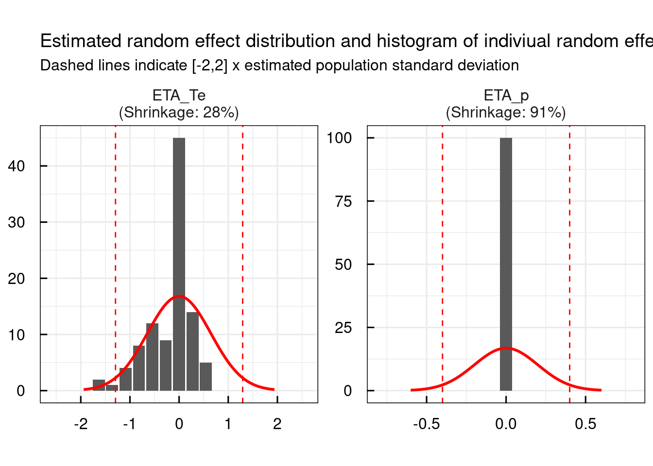 And a VPC for the TTE data (both on linear and log Y axis):
11.2.4 Weibull with delay
IQRtteProject(
  model           = "Weibull",
  comment         = "Weibull with delay",
  repeated        = FALSE,
  delay           = TRUE,
  modelSpec       = list(
    POPvalues0 = c(Te=319,p=11,del=10),
    IIVvalues0 = c(Te=0.5,p=0.2,del=0.2),
    IIVestimate = c(Te=1,p=2,del=2)
  ),
  data            = data,
  projectPath     = "material/01-04a-X2-TTE/MODEL_02",
  algOpt.K1       = 50,
  algOpt.K2       = 20
)
## IQRtteProject: material/01-04a-X2-TTE/MODEL_02
## Project has not been run yet (most likely)11.2.5 Exponential
IQRtteProject(
  model           = "Exponential",
  comment         = "Exponential",
  repeated        = FALSE,
  delay           = FALSE,
  modelSpec       = list(
    POPvalues0 = c(Te=319)
  ),
  data            = data,
  projectPath     = "material/01-04a-X2-TTE/MODEL_03",
  algOpt.K1       = 50,
  algOpt.K2       = 20
)
## IQRtteProject: material/01-04a-X2-TTE/MODEL_03
## Project has not been run yet (most likely)11.2.6 Exponential with delay
IQRtteProject(
  model           = "Exponential",
  comment         = "Exponential with delay",
  repeated        = FALSE,
  delay           = TRUE,
  modelSpec       = list(
    POPvalues0 = c(Te=319,del=56),
    IIVvalues0 = c(Te=0.5,del=0.2),
    IIVestimate = c(Te=1,del=2)
  ),
  data            = data,
  projectPath     = "material/01-04a-X2-TTE/MODEL_04",
  algOpt.K1       = 50,
  algOpt.K2       = 20
)
## IQRtteProject: material/01-04a-X2-TTE/MODEL_04
## Project has not been run yet (most likely)11.2.7 Gompertz
IQRtteProject(
  model           = "Gompertz",
  comment         = "Gompertz",
  repeated        = FALSE,
  delay           = FALSE,
  modelSpec       = list(
    POPvalues0 = c(Te=300,k=1e-8),
    IIVvalues0 = c(Te=0.5,k=0.2),
    IIVestimate = c(Te=1,k=2)
  ),
  data            = data,
  projectPath     = "material/01-04a-X2-TTE/MODEL_05",
  algOpt.K1       = 50,
  algOpt.K2       = 20
)
## IQRtteProject: material/01-04a-X2-TTE/MODEL_05
## Project has not been run yet (most likely)11.2.8 Gompertz with delay
IQRtteProject(
  model           = "Gompertz",
  comment         = "Gompertz with delay",
  repeated        = FALSE,
  delay           = TRUE,
  modelSpec       = list(
    POPvalues0 = c(Te=319,k=1e-8,del=10),
    IIVvalues0 = c(Te=0.5,k=0.2,del=0.2),
    IIVestimate = c(Te=1,k=2,del=2)
  ),
  data            = data,
  projectPath     = "material/01-04a-X2-TTE/MODEL_06",
  algOpt.K1       = 50,
  algOpt.K2       = 20
)
## IQRtteProject: material/01-04a-X2-TTE/MODEL_06
## Project has not been run yet (most likely)11.2.9 Log-logistic
IQRtteProject(
  model           = "Log-logistic",
  comment         = "Log-logistic",
  repeated        = FALSE,
  delay           = FALSE,
  modelSpec       = list(
    POPvalues0 = c(Te=319,s=13),
    IIVvalues0 = c(Te=0.5,s=0.2),
    IIVestimate = c(Te=1,s=2)
  ),
  data            = data,
  projectPath     = "material/01-04a-X2-TTE/MODEL_07",
  algOpt.K1       = 50,
  algOpt.K2       = 20
)
## IQRtteProject: material/01-04a-X2-TTE/MODEL_07
## Project has not been run yet (most likely)11.3 Joint models
Several things can be understood under “Joint” modeling. A longitudinal PK/PD model can be built in a joint fashion if both PK and PD parameters are estimated at the same time based on PK and PD observations. Joint modeling also could mean to combine longitudinal and time-to-event (TTE) models.
IQR Tools allows both:
- Longitudinal joint modeling is covered here
- Joint longitudinal and TTE modeling is covered below
11.3.1 Longitudinal + TTE
From the model description perspective longitudinal + TTE models can be represented by an IQRnlmeProject. What is required is that the structural model defines a variable that is interpreted as hazard function for the TTE part and assigns it to an output (OUTPUT1, OUTPUT2, etc.) variable.
When defining an NLME project using the IQRnlmeEst() function, the only difference to normal longitudinal modeling is that the errorModel argument needs to be defined differently. In the following an example for a joint model with three observables (PK, biomarker, event) is given
errorModel = list(
  OUTPUT1 = c("absrel",1,0.3),   # PK additive-proportional error model
  OUTPUT2 = c("rel",0.2),        # PD proportional error model
  OUTPUT3 = c("event","hazard")  # Event outcome defined by "event". "hazard" defines the hazard variable in the model
)
Refer to the Chapter about longitudinal NLME modeling for more information as, except for the small change in the error model definition, all is applicable.
11.3.2 Data format
The data format is the same as for longitudinal NLME modeling (see here). TTE observations need to be added into this format by defining the time to event information according to the MONOLIX format documented here.