8 Analysis dataset preparation
IQR Tools implements functionality to facilitate the creation of analysis or modeling datasets based on a general dataset format. The general dataset format aims to at least contain a minimum if inforamtion required and - at the same time - to be flexible to store all information that is relevant for the analysis.
The functions provided by IQRtools enable a traceable programming of the analysis data set. Metadata (e.g., covariate value units, or covariate category labels) is retained and available for documentation and producing meaningful graphs and tables. When manipulating the data for a particular task, e.g., removal of outliers, imputing covariates, log files are written.
In a first section (Example workflow) of this chapter a basic example for establishing a analysis dataset in the following steps is given:
- Dataset specification of origin
- Import to the IQRdataGENERAL format
- Graphical data exploration
- Cleaning the data to establish analysis dataset
- Export to .csv and .xpt
The second section, (Further options) discusses more features for the following steps with which the basic workflow can be customized.
- Settings for dataset import
- Statistical exploration
- Graphical exploration
8.1 Example workflow
8.1.1 Original dataset in general row-based format
In our example, the source data contains data from a single ascending dose study in healthy male subjects that should be prepared for a population PK analysis. The dataset is provided as a comma separated file:
# Define dataset location
dataFile <- "material/01-01-DataProgAnal/dataSource01.csv"
sourceData <- read.csv(dataFile)| USUBJID | TRTNAME | TIME | NT | TIMEUNIT | NAME | VALUE | VALUETXT | UNIT | LLOQ | ROUTE | CENTER | VISIT | STUDY |
|---|---|---|---|---|---|---|---|---|---|---|---|---|---|
| IQ00701-0100-0001 | Placebo | -167.88 | -168.00 | Hours | Age | 34 | . | Years | . | . | 100 | 1 | FIH |
| IQ00701-0100-0001 | Placebo | -167.88 | -168.00 | Hours | Gender | 1 | male | . | . | . | 100 | 1 | FIH |
| IQ00701-0100-0001 | Placebo | -1.00 | -1.00 | Hours | Bodyweight | 89 | . | kg | . | . | 100 | 2 | FIH |
| IQ00701-0100-0001 | Placebo | -1.00 | -1.00 | Hours | Height | 185 | . | cm | . | . | 100 | 2 | FIH |
| IQ00701-0100-0001 | Placebo | 23.00 | 23.00 | Hours | Height | 200 | . | cm | . | . | 100 | 2 | FIH |
| IQ00701-0100-0001 | Placebo | 39.00 | 39.00 | Hours | Height | 250 | . | cm | . | . | 100 | 2 | FIH |
| IQ00701-0100-0001 | Placebo | -0.08 | -0.08 | Hours | Plasma concentration IQ0815 | 0 | . | ug/mL | 0.001 | . | 100 | 2 | FIH |
| IQ00701-0100-0001 | Placebo | 0.00 | 0.00 | Hours | Dose IQ0815 | 0 | . | mg | . | oral | 100 | 2 | FIH |
| IQ00701-0100-0001 | Placebo | 0.08 | 0.08 | Hours | Plasma concentration IQ0815 | 0 | . | ug/mL | 0.001 | . | 100 | 2 | FIH |
| IQ00701-0100-0001 | Placebo | 0.25 | 0.25 | Hours | Plasma concentration IQ0815 | 0 | . | ug/mL | 0.001 | . | 100 | 2 | FIH |
| IQ00701-0100-0002 | 1mg oral single dose | -167.35 | -168.00 | Hours | Age | 29 | . | Years | . | . | 100 | 1 | FIH |
| IQ00701-0100-0002 | 1mg oral single dose | -167.35 | -168.00 | Hours | Gender | 1 | male | . | . | . | 100 | 1 | FIH |
The source dataset contains all information (doses, observations, covariates) in a row-based format and has preserved column names used for the data import in IQR Tools (see table below for a description of the columns of the example dataset). Of the columns in the data only seven (written in bold) are required, but there exist more preserved column names such as “STUDY”, “PART”, or “COMPOUND” to cover the typical information used in pharmacometric or systems pharamacology analyses. The general dataset format is described in detail in the chapter General Dataset Format
An important column is the NAME column identifying which type of event is recorded, e.g., whether the row reports an dosing event, measured plasma concentration value or the age of the subject.
Typical entries for these example could be “Aspririn dose”, “Aspirin concentration”, or “Age at screening visit”.
The VALUE column exclusively contains numerical values.
For categorical covariates the VALUETXT column is used instead or in addition to note the category value, e.g., “yes”/“no” or “red”/“blue”/“green”.
| Column | Description |
|---|---|
| USUBJID | Unique subject identifier |
| TRTNAME | Name of actual treatment given to subject |
| TIME | (NUMERIC) Actual time of event relative to first dose administration |
| NT | (NUMERIC) Nominal event time |
| TIMEUNIT | Unit of all numeric time definitions in the dataset (HOURS, MINUTES, DAYS, SECONDS, WEEKS, MONTHS, YEARS) |
| NAME | Unique short name of event |
| VALUE | (NUMERIC) Value of event defined by NAME |
| VALUETXT | Text version of value (If VALUETXT is defined, VALUE can be undefined and is used to code categorical information |
| UNIT | Unit of the value reported in the VALUE column |
| LLOQ | (NUMERIC) Lower limit of quantification for event defined by NAME (value only interpreted for observation events) |
| ROUTE | Route of administration (e.g., IV,SUBCUT,ORAL,TOPICAL) (value only interpreted for dosing events) |
| CENTER | Center number |
| VISIT | Visit number |
8.1.2 Import as IQRdataGENERAL format
To create an analysis dataset, we need to reformat the dataset and add columns needed for the model-based analysis:
- Numerical columns need to be created
- to discriminate dosing from observation records,
- to identify different observation and dosing types, and
- to flag whether records are valid, missing or out of the measureable range
- Covariates need to be provided in (numerical) columns
Based on the NAME column, we can specify which records are dosing information, observations, and covariate information.
For the dosing and observation records, they only need to be listed in a vector.
For the covariate records, we need to have a named vector.
The names are used as the column names of the covariate columns that will be created.
# Define the names (NAME column) of the records you want to consider as dose records
doseNAMES <- "Dose IQ0815"
# Define the names (NAME column) of the records you want to consider as observation records
obsNAMES <- "Plasma concentration IQ0815"
# Define the CONTINUOUS covariate columns (time INDEPENDENT)
cov0 <- c(
  WT0  = "Bodyweight",          # COLNAME = "NAME of the event"
  AGE0 = "Age",
  HT0  = "Height"
)
# Define the CATEGORICAL covariate columns (time INDEPENDENT) that you want to generate
# from event records in the general dataset
cat0 <- c(
  SEX  = "Gender"
)
# Convert general dataset as an IQRdataGENERAL object
data1 <- IQRdataGENERAL(input=dataFile,
                        doseNAMES=doseNAMES, obsNAMES=obsNAMES,
                        cov0=cov0,cat0=cat0)
The resulting data object data1 contains additional columns that are needed for model-based anylsis.
Some important columns that have been created are
- the column
EVIDindicating dosing events (EVID = 1) and observarion records (EVID = 0), - the column
YTYPEdiscriminating different observation types, - the column
ADMdiscriminating different dosing types, - the column
AMTto annotate dosing amount, - the column
MDVflagging missing data values (MDV = 1), - the column
CENSflagging data values outside the measurable range (e.g.,CENS = 1for BLQ values) - the column
IXGDFwith a unique record number for each row of the dataset.
The covariate columns WT0, HT0, AGE0, and SEX have been added as well containing numerical values.
| IXGDF | USUBJID | TRTNAME | TIME | TIMEUNIT | VALUE | AMT | EVID | YTYPE | ADM | MDV | CENS | WT0 | HT0 | AGE0 | SEX | |
|---|---|---|---|---|---|---|---|---|---|---|---|---|---|---|---|---|
| 5 | 7 | IQ00701-0100-0001 | Placebo | -0.08 | HOURS | 0 | 0 | 0 | 1 | 0 | 1 | 0 | 89 | 185 | 34 | 1 |
| 6 | 8 | IQ00701-0100-0001 | Placebo | 0.00 | HOURS | 0 | 0 | 1 | 0 | 1 | 1 | 0 | 89 | 185 | 34 | 1 |
| 7 | 9 | IQ00701-0100-0001 | Placebo | 0.08 | HOURS | 0 | 0 | 0 | 1 | 0 | 1 | 0 | 89 | 185 | 34 | 1 |
| 8 | 10 | IQ00701-0100-0001 | Placebo | 0.25 | HOURS | 0 | 0 | 0 | 1 | 0 | 1 | 0 | 89 | 185 | 34 | 1 |
| 15 | 15 | IQ00701-0100-0002 | 1mg oral single dose | 0.00 | HOURS | 1 | 1 | 1 | 0 | 1 | 1 | 0 | 65 | 186 | 29 | 1 |
| 20 | 20 | IQ00701-0100-0003 | 1mg oral single dose | -0.08 | HOURS | 0 | 0 | 0 | 1 | 0 | 1 | 0 | 80 | 180 | 28 | 1 |
| 21 | 21 | IQ00701-0100-0003 | 1mg oral single dose | 0.00 | HOURS | 1 | 1 | 1 | 0 | 1 | 1 | 0 | 80 | 180 | 28 | 1 |
| 22 | 22 | IQ00701-0100-0003 | 1mg oral single dose | 0.08 | HOURS | 0 | 0 | 0 | 1 | 0 | 1 | 0 | 80 | 180 | 28 | 1 |
| 23 | 23 | IQ00701-0100-0003 | 1mg oral single dose | 0.25 | HOURS | 0 | 0 | 0 | 1 | 0 | 0 | 0 | 80 | 180 | 28 | 1 |
| 24 | 24 | IQ00701-0100-0003 | 1mg oral single dose | 0.50 | HOURS | 0 | 0 | 0 | 1 | 0 | 0 | 0 | 80 | 180 | 28 | 1 |
| 25 | 25 | IQ00701-0100-0003 | 1mg oral single dose | 1.00 | HOURS | 0 | 0 | 0 | 1 | 0 | 0 | 0 | 80 | 180 | 28 | 1 |
| 26 | 26 | IQ00701-0100-0003 | 1mg oral single dose | 2.00 | HOURS | 0 | 0 | 0 | 1 | 0 | 0 | 0 | 80 | 180 | 28 | 1 |
The variable data1 adopted the class IQRdataGENERAL that stores metadata in its attributes.
Amongst others, the attributes store the information on units, category and covariate names and can be called using the convenience functions covInfo() and catInfo().
Importantly, if present in the source data, the columns STUDY and TRTNAME containing character values covariate columns
were used to create covariate columns STUDYN and TRT containing numerical values.
| COLNAME | NAME | UNIT | TIME.VARYING |
|---|---|---|---|
| WT0 | Bodyweight | kg | FALSE |
| AGE0 | Age | Years | FALSE |
| HT0 | Height | cm | FALSE |
| COLNAME | NAME | UNIT | VALUETXT | VALUES | TIME.VARYING |
|---|---|---|---|---|---|
| SEX | Gender | NA | male | 1 | FALSE |
| STUDYN | Study |
|
FIH,FIH extension | 1,2 | FALSE |
| TRT | TRTNAME |
|
Placebo,1mg oral single dose,2mg oral single dose,5mg oral single dose,10mg oral single dose,20mg oral single dose,50mg oral single dose,100mg oral single dose,200mg oral single dose | 9,3,6,8,2,5,7,1,4 | FALSE |
Using the summary function useful information on the data is displayed. In addition, data integrity checks are performed.
##    INFO                                          | NAME                        | VALUE
##    ---------------------------------------------------------------------------------------------------------------------------------
##    Dose events                                   | Dose IQ0815                 | Ntotal: 48,  Nindiv (min/median/max): 1/1/1)
##    Observation events (all)                      | Plasma concentration IQ0815 | Ntotal: 543,  Nindiv (min/median/max): 3/12/12)
##    Observation events (MDV=0)                    | Plasma concentration IQ0815 | Ntotal: 410,  Nindiv (min/median/max): 5/10/11)
##    Doses AMT=0 present                           | ALL dose events             | TRUE (N=1)
##    Placebo subjects present (AMT=0 or no doses)  | ALL dose events             | TRUE (N=1)
##    IGNORED (MDV=1) observation records present   | ALL observation events      | TRUE (N=133)
##    Subjects without observations (MDV=0) present | ALL observation events      | TRUE (N=3)
##    Total BLLOQ information                       | Plasma concentration IQ0815 | N=133 / 24.5%
##    Max % BLLOQ values in a subject               | Plasma concentration IQ0815 | 8.33%
##    BLLOQ handling method                         | All observation events      | M1
##    NLME columns containing NA                    | All events                  | WT0, AGE0, HT0, SEX
##    Issues present in the data                    | Minor                       | YES (see text below the table for more information)
##    Issues present in the data                    | Warnings                    | NONE
##    Issues present in the data                    | Errors                      | NONE
##
##
## IQRoutputTable object
##
## MINOR issues in the dataset that might be addressed
## ===================================================
## SUBJECT LEVEL (IQ00701-0100-0005): Subject has records of NAME "Plasma concentration IQ0815" at same TIME pointsThe summary and checks help to detect issues in the dataset that should be fixed before an analysis starts. In this example, there is only one placebo subject, but there are 3 individuals without any observation records. Thus, we may want to remove these individuals as well as a duplicated plasma record for subject “IQ00701_0100_0005”. Also, the covariate columns contain NA values and we probably need to impute values for some individuals.
8.1.3 Source data exploration
An recommended step before any data analysis or modeling activity is to explore the data visually.
IQR Tools provides a range of standard plotting function.
Here, we make use of two of them, the function plotSpaghetti_IQRdataGENERAL() producing line plots per treatment group that is very useful to get an overview on the observation time courses and the function plotIndiv_IQRdataGENERAL() producing much more detailed plots for evry individual in a pdf file.
## Warning: `aes_string()` was deprecated in ggplot2 3.0.0.
## ℹ Please use tidy evaluation idioms with `aes()`.
## ℹ See also `vignette("ggplot2-in-packages")` for more information.
## ℹ The deprecated feature was likely used in the IQRtools package.
##   Please report the issue at <https://github.com/IntiQuan/IQRtools/issues>.
## This warning is displayed once per session.
## Call `lifecycle::last_lifecycle_warnings()` to see where this warning was generated.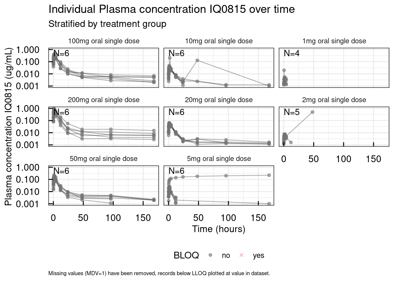
# Generation of a pdf file containing detailed plots for each individual
plotIndiv_IQRdataGENERAL(data1, filename = "material/01-01-DataProgAnal/IndivPlots01.pdf")
From the overview plot we can see that one subject who received 5mg of IQ0815 has a implausible PK profile.
Also, we can spot some outlying records.
The detailed individual plots in the pdf file help to exactly identify the subject with implausible observations and the outlying records:
The plots display the unique subject identifiers, all observations and dosing records as well as the treatment group name.
The observation records are labelled with the unique record identifier IXGDF.
8.1.4 Cleaning to create an analysis dataset
Based on the data exploration, we want to clean the dataset before finally producing the modeling dataset.
Specification of records to be removed
Named lists are created containing either unique subject identifiers (USUBJID) for removing all data from specific subjects or
unique record identifiers (IXGDF) for removing particular records.
The list names can is to annotate the reason for removal.
Specification of covariate imputation
To impute covariates, we use names vectors for continuous and categorical covaraites respectively. The values given will be imputed for all missing covariates. For the continuous covariates, it is also possible to provide suitable function names like “mean” or “median” to calculat the imputation value based on the available values.
Perform documented dataset cleaning
For generating a cleaned analysis dataset, the function clean_IQRdataGENERAL() is used.
It not only accepts the information on data removal or covariate imputation, but has more functionality and options.
In this example, the method to handle BLLOQ data is chosen (methodBLLOQ = "M3"), ignored records are decided to be kept in the dataset (FLAGrmIGNOREDrecords = FALSE), but the placebo subjects are removed (FLAGrmPlacebo = TRUE).
Very importantly, information on the cleaning process is written to the folder specified as pathname input argument.
8.1.5 Export
To make the dataset available for parameter estimation with NONMEM or MONOLIX,
it is exported with the function exportNLME_IQRdataGENERAL().
In this step, some adjustments to the data are done, e.g., removing spaces in character strings, such that the data set is accepted by
the softwares.
# Export the NLME data set with BLQ method M3
exportNLME_IQRdataGENERAL(data1CleanM3,
                          filename = "material/01-01-DataProgAnal/dataNLME01/data.csv",
                          FLAGxpt = TRUE,
                          FLAGdefine = TRUE)
This function also has some options what export is performed. In any case, there will be a csv-file generated.
However, we can use the option FLAGxpt = TRUE to additionally write an xpt-file and the option FLAGdefine = TRUE
to produce a define file with data set specifications for the analysis dataset. Click
here to download the example define file.
8.2 Workflow customization
8.2.1 Dataset handling
For showing more examples to import a dataset as IQRdataGENERAL object, we load another dataset from file.
Multiple dose or observation types
This data contains dosings of two different drugs and two observations types.
Note that the IQRdataGENERAL() function accepts the path to the source data (see example workflow above) but also the
loaded data frame as input.
# Dose records
doseNAMES <- c("Dose Z","Dose X")
# Observation records
obsNAMES <- c("Plasma concentration Z","Efficacy marker")
# Import as IQRdataGENERAL
data2 <- IQRdataGENERAL(dataSource2, doseNAMES = doseNAMES, obsNAMES = obsNAMES)| USUBJID | TRTNAME | NAME | TIME | VALUE | AMT | EVID | YTYPE | ADM | |
|---|---|---|---|---|---|---|---|---|---|
| 1 | ZY1000101066 | SD IV 15 mg/kg | Efficacy marker | -7.1118056 | 21.152 | 0 | 0 | 2 | 0 |
| 3 | ZY1000101066 | SD IV 15 mg/kg | Dose X | 0.0000000 | 918.000 | 918 | 1 | 0 | 2 |
| 4 | ZY1000101066 | SD IV 15 mg/kg | Plasma concentration Z | 0.0826389 | 998.001 | 0 | 0 | 1 | 0 |
| 6 | ZY1000101066 | SD IV 15 mg/kg | Plasma concentration Z | 16.2076389 | 159.399 | 0 | 0 | 1 | 0 |
| 7 | ZY1000101066 | SD IV 15 mg/kg | Plasma concentration Z | 29.2006944 | 119.400 | 0 | 0 | 1 | 0 |
| 8 | ZY1000101066 | SD IV 15 mg/kg | Plasma concentration Z | 42.1701389 | 42.201 | 0 | 0 | 1 | 0 |
| 9 | ZY1000101066 | SD IV 15 mg/kg | Efficacy marker | 112.2256944 | 22.223 | 0 | 0 | 2 | 0 |
| 10 | ZY1000101067 | SD IV 15 mg/kg | Efficacy marker | -13.8138889 | 23.043 | 0 | 0 | 2 | 0 |
| 12 | ZY1000101067 | SD IV 15 mg/kg | Dose X | 0.0000000 | 1311.000 | 1311 | 1 | 0 | 2 |
| 13 | ZY1000101067 | SD IV 15 mg/kg | Plasma concentration Z | 0.0972222 | 1362.000 | 0 | 0 | 1 | 0 |
| 15 | ZY1000101067 | SD IV 15 mg/kg | Plasma concentration Z | 15.0736111 | 176.199 | 0 | 0 | 1 | 0 |
| 16 | ZY1000101067 | SD IV 15 mg/kg | Plasma concentration Z | 29.2506944 | 100.599 | 0 | 0 | 1 | 0 |
Time-varying covariates
Time-varying covariates are defined analogue to time-independent covariates.
The PD observations are here used once as baseline covariate as well as time-dependent covariate.
In the first case, all records are used in the covariate column according to the time of the observation records they are mapped onto.
In case it is used as time independent covariate, the baseline value per individual (defined by columns BASE, SCREEN, or pre-first dose records, for details see ?IQRdataGENERAL)
will be mapped to the observations.
# Define the CONTINUOUS covariate columns (time INDEPENDENT)
cov0 <- list(
  PDbase  = "Efficacy marker"
)
# Define the CONTINUOUS covariate columns (time DEPENDENT)
covT <- list(
  PDcont  = "Efficacy marker"
)
# Define the CATEGORICAL covariate columns (time INDEPENDENT)
cat0 <- list(
  SEX  = "Gender"
)
# Define the CATEGORICAL covariate columns (time DEPENDENT)
catT <- list(
  HSTAT   = "Health status"
)
# Import to IQRdataGENERAL object
data2 <- IQRdataGENERAL(dataSource2, doseNAMES = doseNAMES, obsNAMES = "Plasma concentration Z",
                        cov0 = cov0, cat0 = cat0,
covT = covT, catT = catT)| USUBJID | TRTNAME | NAME | TIME | VALUE | AMT | EVID | YTYPE | ADM | PDbase | PDcont | SEX | HSTAT | |
|---|---|---|---|---|---|---|---|---|---|---|---|---|---|
| 3 | ZY1000101066 | SD IV 15 mg/kg | Dose X | 0.0000000 | 918.000 | 918 | 1 | 0 | 2 | 21.152 | 21.152 | NA | 3 |
| 4 | ZY1000101066 | SD IV 15 mg/kg | Plasma concentration Z | 0.0826389 | 998.001 | 0 | 0 | 1 | 0 | 21.152 | 21.152 | NA | 3 |
| 6 | ZY1000101066 | SD IV 15 mg/kg | Plasma concentration Z | 16.2076389 | 159.399 | 0 | 0 | 1 | 0 | 21.152 | 21.152 | NA | 3 |
| 7 | ZY1000101066 | SD IV 15 mg/kg | Plasma concentration Z | 29.2006944 | 119.400 | 0 | 0 | 1 | 0 | 21.152 | 21.152 | NA | 3 |
| 8 | ZY1000101066 | SD IV 15 mg/kg | Plasma concentration Z | 42.1701389 | 42.201 | 0 | 0 | 1 | 0 | 21.152 | 21.152 | NA | 3 |
| 12 | ZY1000101067 | SD IV 15 mg/kg | Dose X | 0.0000000 | 1311.000 | 1311 | 1 | 0 | 2 | 23.043 | 23.043 | NA | 2 |
| 13 | ZY1000101067 | SD IV 15 mg/kg | Plasma concentration Z | 0.0972222 | 1362.000 | 0 | 0 | 1 | 0 | 23.043 | 23.043 | NA | 2 |
| 15 | ZY1000101067 | SD IV 15 mg/kg | Plasma concentration Z | 15.0736111 | 176.199 | 0 | 0 | 1 | 0 | 23.043 | 23.043 | NA | 3 |
| 16 | ZY1000101067 | SD IV 15 mg/kg | Plasma concentration Z | 29.2506944 | 100.599 | 0 | 0 | 1 | 0 | 23.043 | 23.043 | NA | 3 |
| 17 | ZY1000101067 | SD IV 15 mg/kg | Plasma concentration Z | 42.1562500 | 57.201 | 0 | 0 | 1 | 0 | 23.043 | 23.043 | NA | 3 |
| 21 | ZY1000101068 | SD IV 15 mg/kg | Dose X | 0.0000000 | 0.000 | 0 | 1 | 0 | 2 | 23.364 | 23.364 | NA | 4 |
| 26 | ZY1000101069 | SD IV 15 mg/kg | Plasma concentration Z | -0.0013889 | 0.933 | 0 | 0 | 1 | 0 | 16.993 | 16.993 | NA | 1 |
Existing covariate columns
Datasets may also contain (numerical) covariate columns instead of row-records for covariates. In this case the user needs to provide the metadata (verbose name, units, mapping of category names and values, …) such that it is added to the covariate information in the attributes.
# Additional CONTINUOUS covariates
covInfoAdd <- list(
  COLNAME      = c("AST0",         "BMI0"),
  NAME         = c("Aspartate transaminase","Body mass index"),
  UNIT         = c("UI/mL",      "kg/m2"),
  TIME.VARYING = c(FALSE,              FALSE)
)
# Additional CATEGORICAL covariates
catInfoAdd <- list(
  COLNAME      = c("FOOD"),
  NAME         = c("Food taken"),
  UNIT         = c("y/n"),
  VALUETXT     = c("No,Yes"),
  VALUES       = c("0,1"),
  TIME.VARYING = c(FALSE)
)
# Import to IQRdataGENERAL object
data2 <- IQRdataGENERAL(dataSource2, doseNAMES = doseNAMES, obsNAMES = obsNAMES,
covInfoAdd = covInfoAdd, catInfoAdd = catInfoAdd)| COLNAME | NAME | UNIT | TIME.VARYING |
|---|---|---|---|
| AST0 | Aspartate transaminase | UI/mL | FALSE |
| BMI0 | Body mass index | kg/m2 | FALSE |
| COLNAME | NAME | UNIT | VALUETXT | VALUES | TIME.VARYING |
|---|---|---|---|---|---|
| FOOD | Food taken | y/n | No,Yes | 0,1 | FALSE |
| STUDYN | Study |
|
Y10,Y1,Y3,Y8 | 2,1,3,4 | FALSE |
| TRT | TRTNAME |
|
SD IV 15 mg/kg,SD IV Placebo,SD IV 1.5 mg/kg,MD IV Placebo,MD IV 5mg/kg,SD or MD IV Placebo,MD IV 15mg/kg | 5,6,4,3,2,7,1 | FALSE |
Existing NLME columns
The input argument FLAGforceOverwriteNLMEcols defines if “NLME” columns that already might be
in the dataset are overwritten (TRUE=default) or not (FALSE).
These NLME columns are the following numeric - NLME tool specific columns: ID, TIMEPOS, TAD, DV, MDV, EVID, CENS, AMT, ADM, TINF, RATE,
YTYPE, and DOSE. Overwritting is good in a sense that these columns will be well-defined and aligned
with the dataspec of IQRtools. Not over-writing them can be useful if the user manually wants to
ensure certain things. But in this case the user should now what to do.
If this flag is set to TRUE than all already existing NLME columns will be overwritten. Non-present ones will be (in both cases) generated based on the default spec.
# Overwriting the NLME columns
data2 <- IQRdataGENERAL(dataSource2, doseNAMES, obsNAMES,FLAGforceOverwriteNLMEcols=TRUE)| USUBJID | TIME | EVID | YTYPE | VALUE | ADM | AMT | |
|---|---|---|---|---|---|---|---|
| 1 | ZY1000101066 | -7.11 | 0 | 2 | 21.15 | 0 | 0 |
| 3 | ZY1000101066 | 0.00 | 1 | 0 | 918.00 | 2 | 918 |
| 4 | ZY1000101066 | 0.08 | 0 | 1 | 998.00 | 0 | 0 |
| 6 | ZY1000101066 | 16.21 | 0 | 1 | 159.40 | 0 | 0 |
| 7 | ZY1000101066 | 29.20 | 0 | 1 | 119.40 | 0 | 0 |
| 8 | ZY1000101066 | 42.17 | 0 | 1 | 42.20 | 0 | 0 |
# Keeping existing NLME columns
data2 <- IQRdataGENERAL(dataSource2, doseNAMES, obsNAMES,FLAGforceOverwriteNLMEcols=FALSE)| USUBJID | TIME | EVID | YTYPE | VALUE | ADM | AMT | |
|---|---|---|---|---|---|---|---|
| 1 | ZY1000101066 | -7.11 | 0 | 2 | 21.15 | 0 | 0 |
| 3 | ZY1000101066 | 0.00 | 1 | 0 | 918.00 | 2 | 918 |
| 4 | ZY1000101066 | 0.08 | 0 | 1 | 998.00 | 0 | 0 |
| 6 | ZY1000101066 | 16.21 | 0 | 1 | 159.40 | 0 | 0 |
| 7 | ZY1000101066 | 29.20 | 0 | 1 | 119.40 | 0 | 0 |
| 8 | ZY1000101066 | 42.17 | 0 | 1 | 42.20 | 0 | 0 |
8.2.2 Import/export options
Export IQRdataGENERAL objects
An IQRdataGENERAL object can be exported with three different functions,
export_IQRdataGENERAL(), exportNLME_IQRdataGENERAL(), or exportSYS_IQRdataGENERAL.
The first will export the dataset without further modifications, the other apply estimation tool
specific modifications (e.g., removal of whitespaces in strings) to be applicable as modeling dataset later on.
All export function generate a .csv file and a .atr file storing the metadata and can additionally generate define files and .xpt files.
With all export functions a zipped file instead of the single files (.csv, .atr, …) can be generated by setting FLAGzip = TRUE.
The exportNLME_IQRdataGENERAL() and exportSYS_IQRdataGENERAL() provide the possibility to
subset the data to specific dosing records and observation records (inputs doseNAMES and obsNAMES) and define columns as regressor variables while exporting the data.
Regressor columns are ordered in the exported dataset as given in the input regressorNames which is crucial for matching regressor variables between data and model for some estimation tools.
Load IQRdataGENERAL object
The load_IQRdataGENERAL() function is used to reload a dataset that was generated by
the export_IQRdataGENERAL(), exportNLME_IQRdataGENERAL(), or exportSYS_IQRdataGENERAL function.
In order for the loading to work the dataex.atr file needs to be present in the same folder as
the .csv file. xpt files are not loaded.
Also zip files can be reloaded.
8.2.3 Cleaning options
The cleaning functions clean_IQRdataGENERAL() is actually a wrapper function for various functions performing different steps during cleaning.
They could be called individually. Please refer to the help for each function for detailed information.
| Function | Description | Control in clean_IQRdataGENERAL | Logfile written |
|---|---|---|---|
| blloq _IQRdataGENERAL | Set the BLLOQ handling method | set by methodBLLOQ |
No |
| setIGNORErecords _IQRdataGENERAL | Set user defined records to IGNORE | optional by setting records |
Yes |
| rmMissingTIMEobsRecords _IQRdataGENERAL | Remove missing observation records with missing TIME | always applied | Yes |
| setMissingDVobsRecordsIGNORE _IQRdataGENERAL | Set missing observation records with missing DV to IGNORE | always applied | Yes |
| rmSubjects _IQRdataGENERAL | Remove user defined subjects | optional by setting subjects |
Yes |
| rmNonTask _IQRdataGENERAL | Remove non-dose and non-observation records | always applied | Yes |
| rmPLACEBO _IQRdataGENERAL | Remove placebo subjects | optional by setting FLAGrmPlacebo |
Yes |
| rmNOobsSUB _IQRdataGENERAL | Removal of subjects without observations | always applied | Yes |
| rmAMT0 _IQRdataGENERAL | Removal of dose records with AMT=0 | always applied | Yes |
| rmIGNOREd _IQRdataGENERAL | Removal of ignored record (MDV=1) | optional by setting FLAGrmIGNOREDrecords |
Yes |
| covImpute _IQRdataGENERAL | Imputation of missing covariates | optional by setting continuousCovs and categoricalCovs |
Yes |
| rmDosePostLastObs _IQRdataGENERAL | Removal of doses post last observation | optional by setting FLAGrmDosePostLastObs |
Yes |
8.2.4 Data exploration
In the Example workflow discussed above some of the IQRtools functions to explore a dataset have been used to visualize and detect issues in the data and get an overview on the contained PK observations. In the following all available data exploration functions are introduced using the the cleaned dataset from the workflow as an example.
Summary tables
Summary tables can be generated for observations (summaryObservations_IQRdataGENERAL()) and for categorical or continuous covariates (summaryCat_IQRdataGENERAL() and summaryCov_IQRdataGENERAL).
The tables can be stratified by a suitable dataset column (stratifyColumn with “STUDY” as default).
Beside the actual content a table title and table footer are defined which can be modified by the user (tableTitle and footerAddText).
They can be further customized by setting the number of digits values are rounded to (SIGNIF) and whether individuals should be termed as “subjects” or “patients” (FLAGpatients).
If a filename is provided, the table is written to that file, otherwise a IQRoutputTable object is returned.
With this flexibility the summary tables are intended to be readily suitable to use in modeling reports in the data exploration section. The exported tables are prepared to be automatically imported to a report using IQReport (see Reporting in Microsoft Word).
Observations
For the observation summary table, numbers of subjects and numbers of observations are listed and subsetted for different criteria (e.g., number of observations below the limit of quantification).
The input obsNames is available if only a subset of the contained observations should be summarized.
In this example, there is only one observation, i.e., the “Plasma concentration IQ0815”.
The first two rows give the numbers per study while the last row contains total counts in the entire dataset.
##    Summary of available observations
##    ===================================================================================================================================================================================================================
##
##    Data          | N subjects* | N samples | N BLOQ samples** | N BLOQ samples post first dose** | N missing observations | N missing time information | N total ignored observations | N samples included in analysis
##    -------------------------------------------------------------------------------------------------------------------------------------------------------------------------------------------------------------------
##    FIH           | 32 / 32     | 384       | 117 (30.5%)      | 85 (22.1%)                       | 0 (0%)                 | 0 (0%)                     | 3 (0.781%)                   | 381 (99.2%)
##    FIH extension | 12 / 12     | 144       | 12 (8.33%)       | 0 (0%)                           | 0 (0%)                 | 0 (0%)                     | 0 (0%)                       | 144 (100%)
##    TOTAL         | 44 / 44     | 528       | 129 (24.4%)      | 85 (16.1%)                       | 0 (0%)                 | 0 (0%)                     | 3 (0.568%)                   | 525 (99.4%)
##    -------------------------------------------------------------------------------------------------------------------------------------------------------------------------------------------------------------------
## N: Number of
## * All subjects / subjects with at least one non missing (MDV==0) sample.
## ** These records are not excluded from the analysis but censored (M3 method).
##
##
## IQRoutputTable object
This summary table contains information about samples before and after first dosing regarding BLQ and zero/non-zero values which is mainly of interest for summarizing PK samples.
These can be neglected setting FLAGpk = FALSE:
##    Summary of available observations
##    ================================================================================================================================================================================
##
##    Data          | N subjects* | N samples | N BLOQ samples** | N missing observations | N missing time information | N total ignored observations | N samples included in analysis
##    --------------------------------------------------------------------------------------------------------------------------------------------------------------------------------
##    FIH           | 32 / 32     | 384       | 117 (30.5%)      | 0 (0%)                 | 0 (0%)                     | 3 (0.781%)                   | 381 (99.2%)
##    FIH extension | 12 / 12     | 144       | 12 (8.33%)       | 0 (0%)                 | 0 (0%)                     | 0 (0%)                       | 144 (100%)
##    TOTAL         | 44 / 44     | 528       | 129 (24.4%)      | 0 (0%)                 | 0 (0%)                     | 3 (0.568%)                   | 525 (99.4%)
##    --------------------------------------------------------------------------------------------------------------------------------------------------------------------------------
## N: Number of
## * All subjects / subjects with at least one non missing (MDV==0) sample.
## ** These records are not excluded from the analysis but censored (M3 method).
##
##
## IQRoutputTable object
Covariates
Continuous covariates are summarized by the mean, standard deviation and range from minimum to maximum value while
the number of individuals in therespective and the percent of total is given for categorical covariates.
Summaries are given stratified defined in the stratification (e.g., stratifyColumns = "TRTNAME"; default: “STUDY”) and a total column can be required (FLAGtotal = TRUE).
##    Summary of demographic and baseline characteristics for continuous information
##    ==============================================================================================================================================================================================================================================================
##
##    Characteristic  | 1mg oral single dose [N=4] | 2mg oral single dose [N=5] | 5mg oral single dose [N=5] | 10mg oral single dose [N=6] | 20mg oral single dose [N=6] | 50mg oral single dose [N=6] | 100mg oral single dose [N=6] | 200mg oral single dose [N=6]
##    --------------------------------------------------------------------------------------------------------------------------------------------------------------------------------------------------------------------------------------------------------------
##    Bodyweight (kg) | 76 (8.49) [68-86]          | 80.2 (8.04) [68-88]        | 73.2 (10.1) [65-90]        | 81 (5.1) [75-88]            | 77 (6.2) [68-87]            | 81.3 (7.79) [74-94]         | 85.5 (5.58) [78-92]          | 77.2 (7.91) [67-91]
##    Age (Years)     | 29.2 (4.19) [25-35]        | 29.4 (1.67) [28-32]        | 29.6 (5.32) [24-36]        | 26.3 (5.32) [18-34]         | 28.8 (3.54) [23-32]         | 30.3 (4.8) [23-35]          | 28.8 (5.78) [21-34]          | 30.3 (5.24) [22-38]
##    Height (cm)     | 178 (7.77) [166-183]       | 177 (2.74) [174-181]       | 175 (2.65) [171-178]       | 179 (3.5) [175-183]         | 180 (6.31) [168-186]        | 179 (3.22) [174-182]        | 181 (4.1) [178-188]          | 176 (3.78) [172-183]
##    --------------------------------------------------------------------------------------------------------------------------------------------------------------------------------------------------------------------------------------------------------------
## N: Number of subjects
## Entries represent: Mean (Standard deviation) [Minimum-Maximum]
##
## IQRoutputTable object## Summary of demographic and baseline characteristics for categorical information
## ==========================================================================================
##
## Characteristic | Category | FIH [N=32] | FIH extension [N=12] | TOTAL [N=44]
## ------------------------------------------------------------------------------------------
## Study | FIH | 32 (100%) | 0 (0%) | 32 (72.7%)
## | FIH extension | 0 (0%) | 12 (100%) | 12 (27.3%)
## TRTNAME | Placebo | 0 (0%) | 0 (0%) | 0 (0%)
## | 1mg oral single dose | 4 (12.5%) | 0 (0%) | 4 (9.09%)
## | 2mg oral single dose | 5 (15.6%) | 0 (0%) | 5 (11.4%)
## | 5mg oral single dose | 5 (15.6%) | 0 (0%) | 5 (11.4%)
## | 10mg oral single dose | 6 (18.8%) | 0 (0%) | 6 (13.6%)
## | 20mg oral single dose | 6 (18.8%) | 0 (0%) | 6 (13.6%)
## | 50mg oral single dose | 6 (18.8%) | 0 (0%) | 6 (13.6%)
## | 100mg oral single dose | 0 (0%) | 6 (50%) | 6 (13.6%)
## | 200mg oral single dose | 0 (0%) | 6 (50%) | 6 (13.6%)
## ------------------------------------------------------------------------------------------
## N: Number of subjects
## Number of subjects in each category and percentage within this category
##
## IQRoutputTable objectStandard graphs
Details on individuals
One example for an indidual detail plot was already shown in the data preparation workflow above.
This function creates a pdf with one page per individual and/or a list of graphs (one list element per individual.)
It displays the observations along with the dose administrations and gives information on subject ID and treatment groups.
Each data point is labeled with the IXGDF number.
The data can be inspected in detail to check correctness of the data and problematic data points spotted and identified easily.
Please refer to the help of this function to look up possible customization (e.g., log-scale, selection of observations to include).
Dosing
The dosing schedule per individual can be inspected using the plotDoseSchedule_IQRdataGENERAL() function.
The individual panels are distributed over multiple pages/graphs accoding to the number of individuals to be plot on one page (NperPage, defaults to 25).
Observations
The sampling schedule per individual can be inspected using the plotSampleSchedule_IQRdataGENERAL() function.
The individual panels are distributed over multiple pages/graphs accoding to the number of individuals to be plot on one page (here set by NperPage = 6).
plotSampleSchedule_IQRdataGENERAL(data1CleanM3, filename = "material/01-01-DataProgAnal/Sampling01.pdf", NperPage = 6)The actual observations can be visualized with plotRange_IQRdataGENERAL() and plotSpaghetti_IQRdataGENERAL().
In both cases, the data will be stratified to panels per treatment group.
The first function provides the median and 90% range from the 5th to the 95th percentile of the data per nomnal time point.
The second function will plot the data points at the actual times connected by lines per subjects.
Besides changing the scale (scale = “log” or “lin”, not shown here), the plots can be subsetted by a stratification column and the non-stratified as well as stratified graphs are provided.
# Median and 90% interval per nominal time point
out <- plotRange_IQRdataGENERAL(data1CleanM3)
out$unstratified$`Plasma concentration IQ0815`
## Warning: No shared levels found between `names(values)` of the manual scale and
## the data's colour values.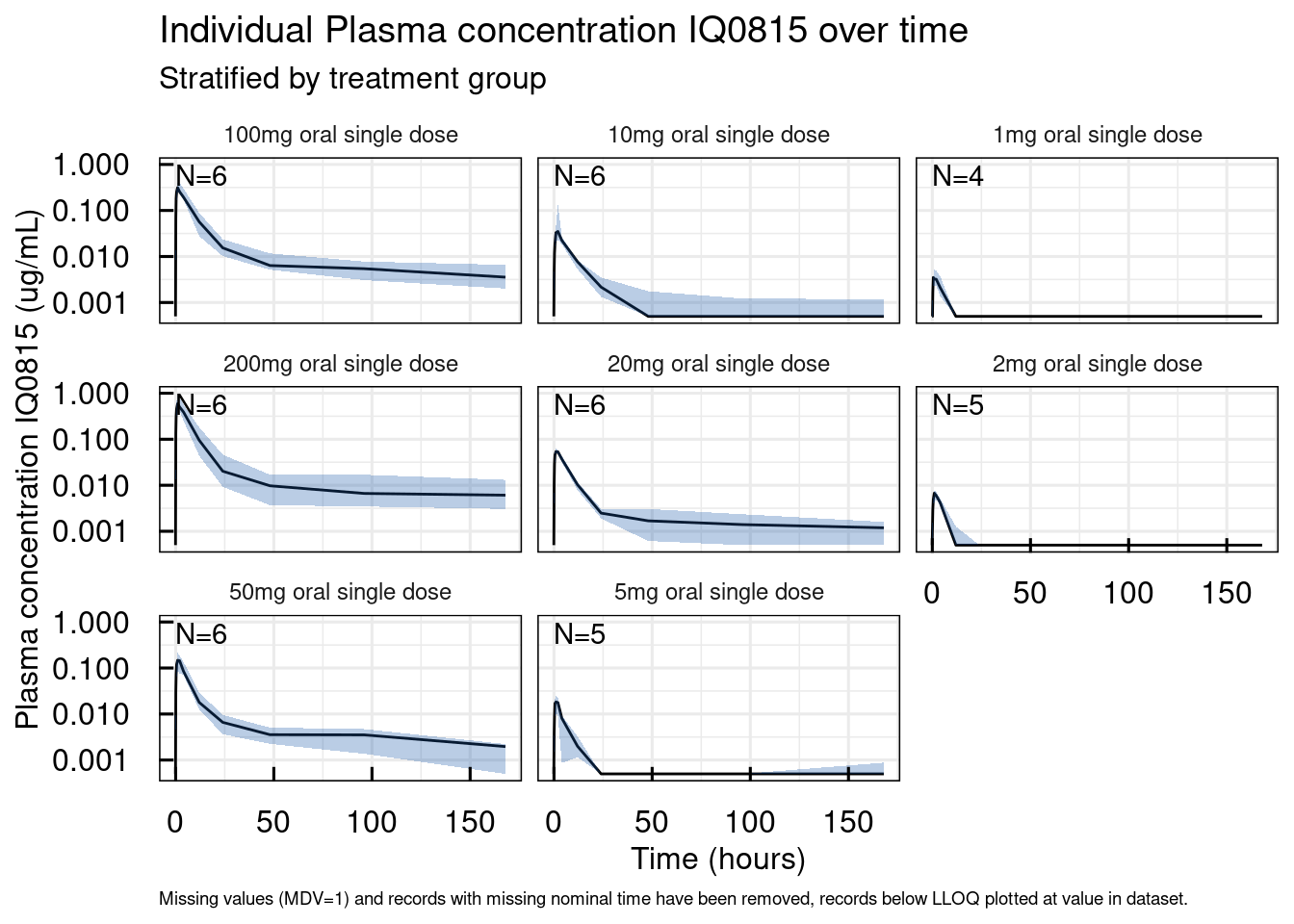
# Lines per idividual
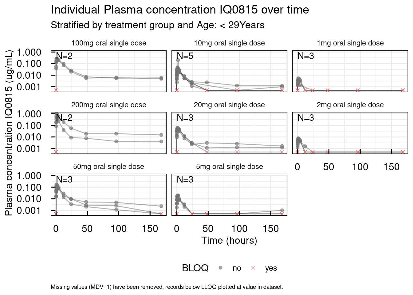
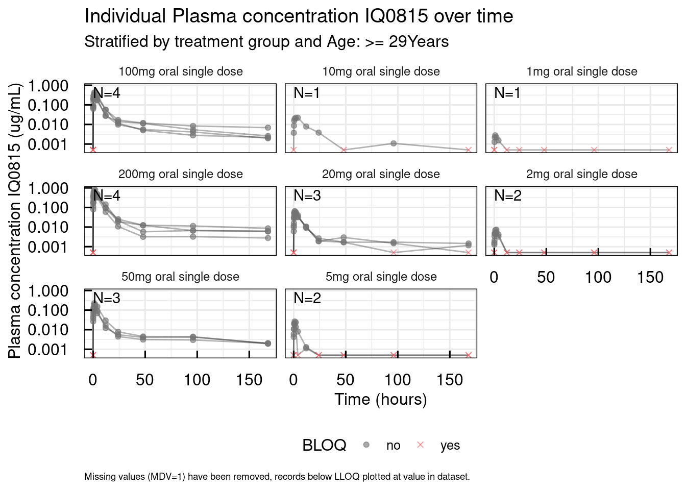
out <- plotSpaghetti_IQRdataGENERAL(data1CleanM3, stratify = "AGE0")
# Unstratified
out$unstratified$`Plasma concentration IQ0815`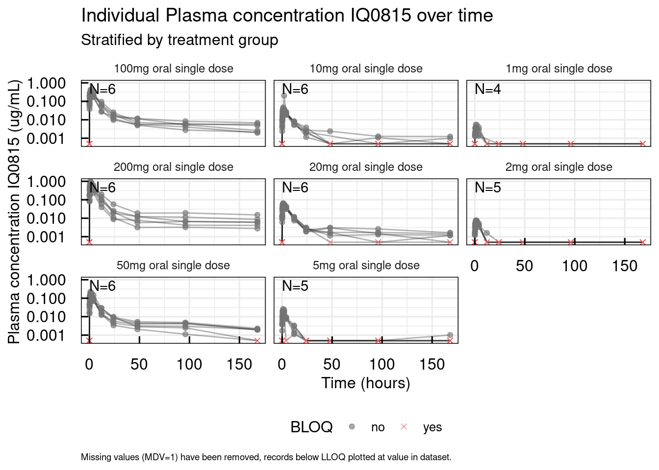
Covariates
The function plotCovDistribution_IQRdataGENERAL() visualizes the distribution of continuous and covariates,
thus being a graphical counterpart to the summaryCov_IQRdataGENERAL() and summaryCat_IQRdataGENERAL() functions.
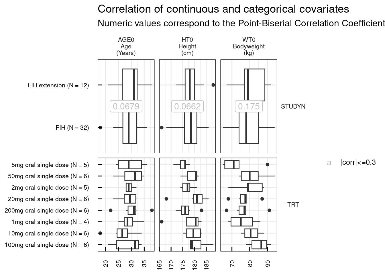
Graphically we can explore also the correlations among continuous covariates (plotCorCov_IQRdataGENERAL()), among categorical covariates (plotCorCat_IQRdataGENERAL()), and between continuous and categorical covariates (plotCorCovCat_IQRdataGENERAL()).
In our example, we make use of the input arguments covNames/catNames to neglect the SEX covariate in the plots as it contains only one category (see summary table above).
# Distribution of continuous and categorical covariates
out <- plotCovDistribution_IQRdataGENERAL(data1CleanM3, covNames = c("STUDYN", "TRT"))
out$categorical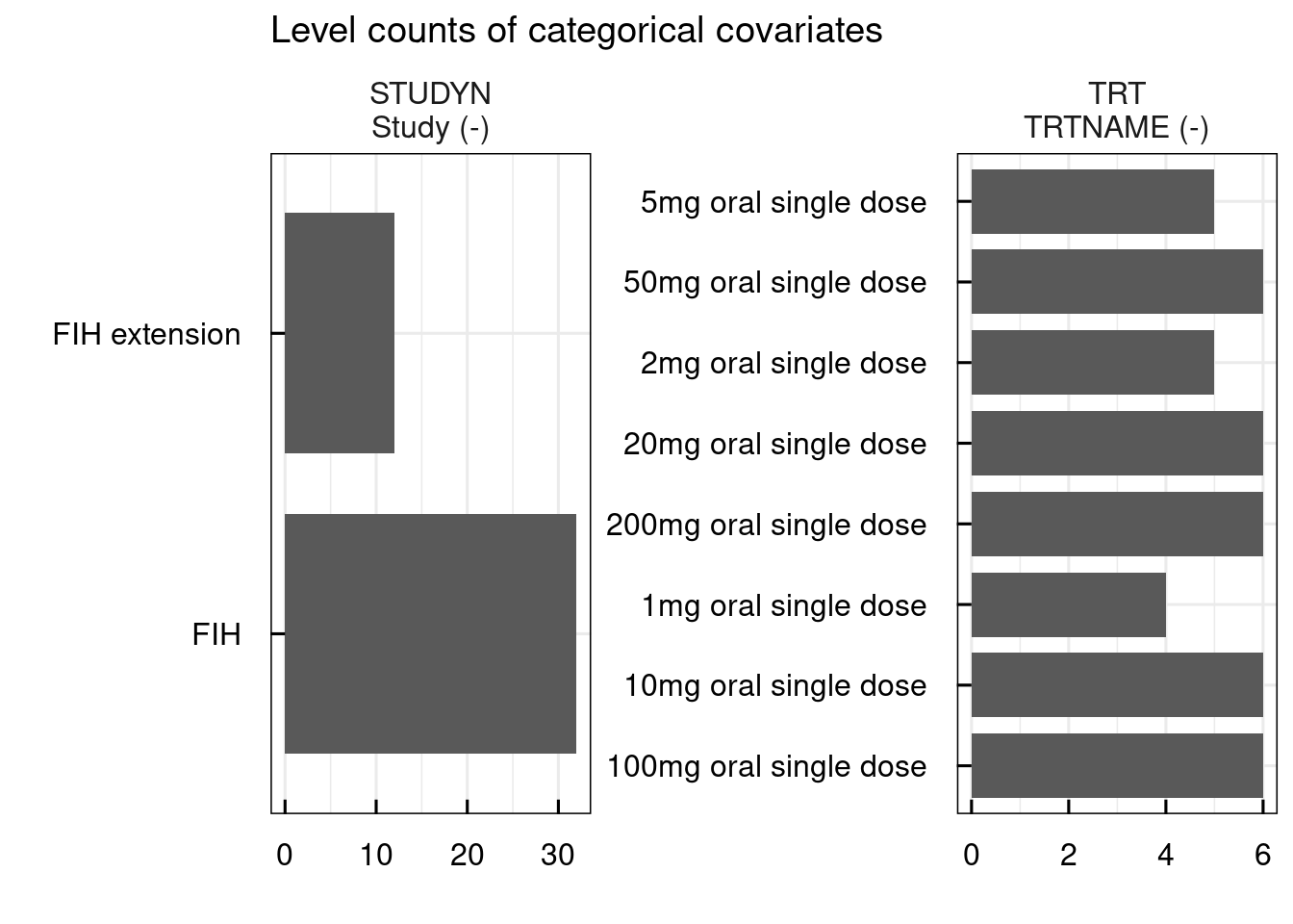
# Correlation of continuous covariates
plotCorCov_IQRdataGENERAL(data1CleanM3,covNames = c("AGE0","WT0","HT0"))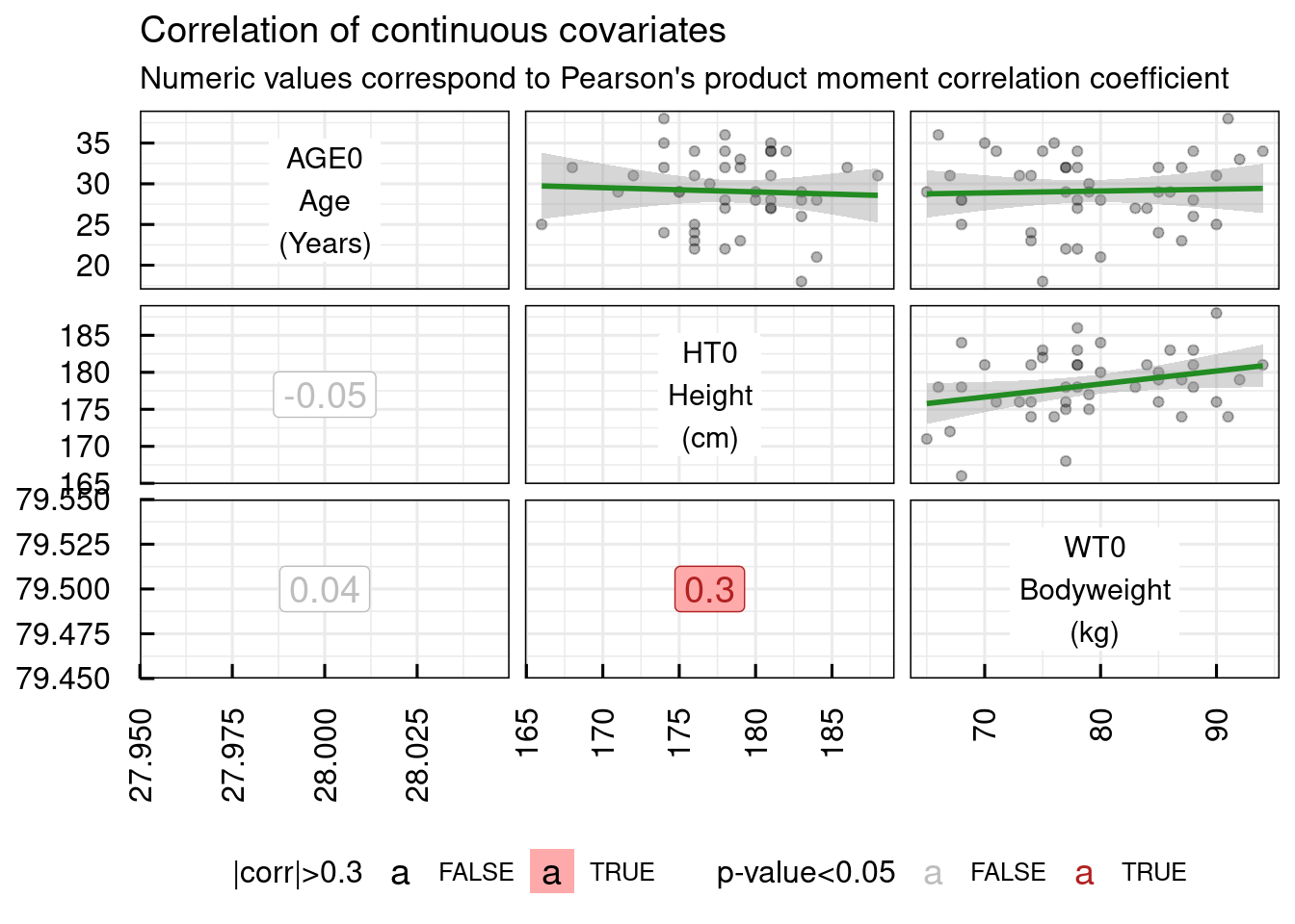
# Correlation of categorical covariates
plotCorCat_IQRdataGENERAL(data1CleanM3, catNames = c("STUDYN", "TRT"))
## Warning in fortify(data, ...): Arguments in `...` must be used.
## ✖ Problematic argument:
## • drop = TRUE
## ℹ Did you misspell an argument name?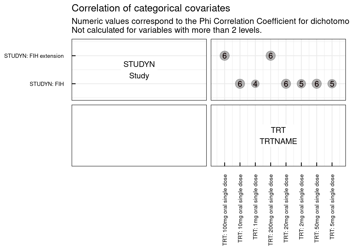
# Correlation of continuous and categorical covariates
plotCorCovCat_IQRdataGENERAL(data1CleanM3, catNames = c("STUDYN", "TRT"))