23 Random sampling of NLME model parameters
This chapter introduces the IQRtools functions for sampling NLME model parameters. Before reading it, it is highly recommended to become familiar with the section Basic terms in chapter General Parameter Format.
Sampling of random parameter values is used to simulate individual phenotypes of patients or other organisms. Here we describe the steps for sampling a random individual value \(X_{i}\) for a model parameter \(X\), as implemented in the family of functions called “NLME parameter sampling API”.
23.1 Input
The input to the API functions represents a GPF file describing the parameter estimates, a data.frame, hereby called “data”, containing individual patient data (such as age and weight) that influence model parameter values, and an argument FLAG_SAMPLE specifying how the sampling is to be done.
23.1.1 Example GPF file
See the Example GPF file section in chapter General Parameter Format.
23.2 Calling the function sampleIndParamValues
set.seed(1)
listResultsSampling <- sampleIndParamValues(
  fileXLS,
  Nsamples = 10,
  FLAG_SAMPLE = 1,
  data = data)
23.2.1 Output
The output of both functions represents an R list with the following members:
| Element | Meaning |
|---|---|
$popParamValues |
a data.frame with a column ID.POP and columns for all population parameter values. For details, see Step 1. |
$sampledData |
a data.frame having Nsample rows representing sampled records from the patient data. For details, see Step 2. |
$typicalIndParamValues |
a data.frame of Nsample * nrow(popParamValues) rows, columns ID.POP and ID, and columns corresponding to the model parameters. The parameter values represent typical individual parameter values taking into account the corresponding covariate values in $sampledData. For details, see Step 3. |
$randomEffects |
a data.frame of the same dimensionality as $typicalIndParamValues containing the random effects sampled from the IIV distribution (in normal units). For details, see Step 4 |
$indParamValues |
a data.frame of the same dimensionality as $typicalIndParamValues containing the (final) individual parameter values in original units. For details, see Step 5 |
$FLAG_SAMPLE |
same as the argument |
$Nsamples |
same as the argument |
23.2.2 Example output
## $sampledData
##    ID      WT0 SEX ID0
## 1   1 17.72027   1   1
## 2   2 20.83697   1   2
## 3   3 20.83697   1   2
## 4   4 17.72027   1   1
## 5   5 16.99424   0   3
## 6   6 16.99424   0   3
## 7   7 20.83697   1   2
## 8   8 16.99424   0   3
## 9   9 20.83697   1   2
## 10 10 17.72027   1   1
##
## $popParamValues
##   ID.POP     Tlag1        ka       CL       Vc       Q1      Vp1 omega(Tlag1)
## 1      1 0.5049329 0.4986161 17.40106 304.8851 75.34485 641.0734    0.2609014
##   omega(ka) omega(CL) omega(Vc) omega(Q1) omega(Vp1) corr(CL,Vc) corr(CL,Q1)
## 1 0.3591658 0.3551205 0.6413351 0.6274387  0.3583025   0.7307295   -0.409266
##   corr(Vc,Q1) corr(CL,Vp1) corr(Vc,Vp1) corr(Q1,Vp1) beta_CL(WT0) beta_Vc(WT0)
## 1  -0.8561186    0.5708827    0.1967233    0.3023412         0.75            1
##   beta_Q1(WT0) beta_Vp1(WT0) beta_CL(SEX_1) error_PROP1 error_ADD1
## 1         0.75             1      0.3006208   0.3672481 0.08932075
##
## $typicalIndParamValues
##    ID.POP ID     Tlag1        ka       CL       Vc       Q1      Vp1
## 1       1  1 0.5049329 0.4986161 8.388086 77.18066 26.88950 162.2856
## 2       1  2 0.5049329 0.4986161 9.471875 90.75544 30.36379 190.8289
## 3       1  3 0.5049329 0.4986161 9.471875 90.75544 30.36379 190.8289
## 4       1  4 0.5049329 0.4986161 8.388086 77.18066 26.88950 162.2856
## 5       1  5 0.5049329 0.4986161 6.018363 74.01842 26.05891 155.6365
## 6       1  6 0.5049329 0.4986161 6.018363 74.01842 26.05891 155.6365
## 7       1  7 0.5049329 0.4986161 9.471875 90.75544 30.36379 190.8289
## 8       1  8 0.5049329 0.4986161 6.018363 74.01842 26.05891 155.6365
## 9       1  9 0.5049329 0.4986161 9.471875 90.75544 30.36379 190.8289
## 10      1 10 0.5049329 0.4986161 8.388086 77.18066 26.88950 162.2856
##
## $randomEffects
##    ID.POP ID       Tlag1          ka           CL          Vc          Q1
## 1       1  1 -0.31950311  0.13289811 -0.000837045 -0.14594396  0.05095890
## 2       1  2 -0.12351088  0.09593276 -0.154858362 -1.38220349  1.40608605
## 3       1  3 -0.16185452 -0.19485466 -0.068739342 -0.18158875  0.42575911
## 4       1  4  0.01098809  0.43382485  0.139912960  0.42733707 -0.44726294
## 5       1  5 -0.23766071  0.41677697 -0.222483016 -0.57826524  0.11298788
## 6       1  6  0.04122992  0.25149282  0.481702950  0.79476163 -0.21487606
## 7       1  7 -0.17078203  0.56993636  0.133085466  0.73838386 -0.85905019
## 8       1  8  0.46108768  0.20058924 -0.196129859 -0.22930960  0.07019425
## 9       1  9  0.18698997 -0.45850830 -0.180897245  0.18295900 -0.48290089
## 10      1 10  0.23746571 -0.20589735  0.031804837  0.04874714  0.06810399
##            Vp1
## 1  -0.03432517
## 2   0.06485870
## 3   0.21861018
## 4   0.13770059
## 5  -0.52375968
## 6   0.57781465
## 7  -0.18662226
## 8  -0.06369727
## 9  -0.34848232
## 10  0.12400321
##
## $indParamValues
##    ID.POP ID     Tlag1        ka        CL        Vc        Q1       Vp1
## 1       1  1 0.3668387 0.5694862  8.381067  66.70000  28.29528 156.80967
## 2       1  2 0.4462657 0.5488193  8.113007  22.78187 123.88289 203.61604
## 3       1  3 0.4294782 0.4103382  8.842658  75.68497  46.47942 237.45724
## 4       1  4 0.5105117 0.7694387  9.647755 118.33103  17.19250 186.24416
## 5       1  5 0.3981245 0.7564326  4.817872  41.51475  29.17604  92.18185
## 6       1  6 0.5261863 0.6411922  9.742700 163.87036  21.02020 277.36592
## 7       1  7 0.4256611 0.8816303 10.820174 189.91037  12.86101 158.34166
## 8       1  8 0.8007215 0.6093700  4.946526  58.85074  27.95383 146.03199
## 9       1  9 0.6087547 0.3152381  7.904480 108.97597  18.73418 134.67912
## 10      1 10 0.6402708 0.4058319  8.659155  81.03621  28.78459 183.71050
##
## $FLAG_SAMPLE
## [1] 1
##
## $Nsamples
## [1] 10
23.3 Covariate adjustment formulae
The covariate adjustment formulae are written in the column “FORMULA” of the estimates sheet. Each formula is associated with an adjustment parameter denoted \(\beta_{X}(C)\), where \(X\) denotes the affected model parameter, and \(C\) refers to the affecting covariate. The formulae are processed differently, depending on the type of the covariate:
- Continuous covariates: the covariate parameters are named “beta_X(C)”, where X is a parameter name and C is a covariate name (see example input files);
- Categorical covariates: the covariate parameters are named “beta_X(C_#)”, where “#” denotes the category (an integer), for which the corresponding formula in the
FORMULAcolumn is to be applied (the formula is not to be applied unless the individual belongs to the “#” category).
23.4 Possible values for FLAG_SAMPLE
| FLAG_SAMPLE | Meaning |
|---|---|
| 0 | Use point estimates of population parameters (do not consider uncertainty) and sample Nsample individual patients based on these. Covariates considered if defined by user and used in model. Please note: population parameters do not take covariates into account! |
| 1 | Sample single set of population parameters from uncertainty distribution and sample Nsample individual patient parameters based on these. Covariates considered if defined by user and used in model. Please note: population parameters do not take covariates into account! |
| 2 | Sample Nsample sets of population parameters from uncertainty distribution. Do not sample from variability distribution and do not take into account covariates (even if user specified). |
| 3 | Use point estimates of population parameters (do not consider uncertainty) Return Nsamples sets of population parameters with covariates taken into account. |
| 4 | Sample single set of population parameters from uncertainty distribution Return Nsamples sets of population parameters with covariates taken into account. |
| 5 | Use point estimates of population parameters (do not consider uncertainty) and sample Nsample individual patients based on these. Covariates considered if defined by user and used in model. Population parameters, typical individual parameters (no IIV, but considering covariates), and individual parameters are returned. |
| 6 | Sample single set of population parameters from uncertainty distribution and sample Nsample individual patient parameters based on these. Covariates considered if defined by user and used in model. Sampled population parameters, typical individual parameters (no IIV, but considering covariates), and individual parameters are returned. |
23.5 Sampling steps
The sampling procedure for obtaining the final individual parameter values consists of five steps described in the following sub-sections.
Note that the main user API for the sampling is the sampleIndParamValues function. The content below shows to some extent
what happens under the hood. Functions that are not typically needed by a normal user are not exported.
23.5.1 Step 1: Sampling of population parameter values
Population parameter values are sampled from the point estimates’ uncertainty distribution. \[ (\vec{X}_{ref,pop},\vec{\omega}_{pop},\vec{\rho}_{pop},\vec{\beta}_{pop},\vec{\sigma}_{pop})=\vec{g}\big[\vec{f}(\hat{\vec{X}},\hat{\vec{\omega}},\hat{\vec{\rho}},\hat{\vec{\beta}},\hat{\vec{\sigma}})+\vec{\epsilon}\sim\mathcal{N}(\vec{0},\Sigma_{unc})\big] \]
Notation:
- \(\vec{X}\): all model parameters (in their original scale);
- \(\vec{\omega}\): IIV standard deviations of all model parameters (in the parameters’ original scale);
- \(\vec{\rho}\): IIV correlations of the model parameter couples’ correlations (in the parameters’ transformed to normal scale);
- \(\vec{\beta}\): all covariate parameters;
- \(\vec{\sigma}\): all residual error parameters;
- \(\hat{\cdot}\): point estimate of \(\cdot\);
- \(\Sigma_{unc}\): uncertainty variance covariance matrix;
- \(\vec{f}(\cdot)\): vectorized function transforming the parameters to normal scale;
- \(\vec{g}(\cdot)\): vectorized function transforming the parameters from normal scale to their original scale.
Example code:
# Create a IQRnlmeParamSpec object for future use (not suitable for reading by humans):
spec <- IQRtools:::specifyParamSampling(fileXLS, Nsamples = 10, FLAG_SAMPLE = 1)
# Get a data.frame of the parameter transformation types
paramTypes <- IQRtools:::getParamTransformationTypes(spec)# Ensure equivalent results with the previous call to sampleIndParamValues
set.seed(1)
popParamValues <- IQRtools:::sampleParamFromUncertainty(spec)
# Check equivalence with the output from calling sampleIndParamValues:
all.equal(listResultsSampling$popParamValues, popParamValues)## [1] TRUE23.5.2 Step 2: Sampling records from the patient data
The sampling of records from the patient data is done using the function sampleIDs. By convention, the behaviour of this function depends on nrow(data) and the value of Nsamples. If nrow(data) == Nsamples, then all rows in data are included (in their original order); if nrow(data)>Nsamples, sampling without replacement from the rows in data is done; if nrow(data)<Nsamples then sampling with replacement is done. The returned data.frame has a column ID set to the integers 1,...,Nsamples. If the original data object did have a column ID, this column is copied as a column ID0 in the returned data.frame.
Example code:
sampledData <- IQRtools:::sampleIDs(data, spec$Nsamples)

# Check equivalence with the output from calling sampleIndParamValues:
all.equal(listResultsSampling$sampledData, sampledData)
## [1] TRUE23.5.3 Step 3: Calculating typical individual parameter values
This is an adjustment of the model parameter values according to the individual’s covariate values and the covariate formulae. \[ \vec{X}_{typ,i}=\vec{\text{Covrt}}(\vec{X}_{ref,pop},C_{\vec{X},1,i},...,\beta_{\vec{X},1,pop},...), \]
Notation:
- \(i\): index of an individual;
- \(\vec{X}_{typ,i}\): typical individual parameter values - fixed effects;
- \(C_{\vec{X},1,i},...\): all covariate values for individual \(i\);
- \(\beta_{\vec{X},1,pop},...\): all covariate parameters;
- \(\vec{\text{Covrt}}(\vec{X}_{ref,pop}, C_{\vec{X},1,i},..., \beta_{\vec{X},1,pop},...)\): vectorized covariate adjustment function.
Example code:
typicalIndParamValues <- IQRtools:::calcTypicalIndParamValues(spec, popParamValues, sampledData)

# Check equivalence with the output from calling sampleIndParamValues:
all.equal(listResultsSampling$typicalIndParamValues, typicalIndParamValues)
## [1] TRUE23.5.4 Step 4: Sampling random effects
\[ \vec{\eta}_{i}\sim\mathcal{N}(\vec{0},\Sigma_{IIV,pop}) \]
Notation:
- \(\vec{\eta}_{i}\): individual random effects;
- \(\Sigma_{IIV,pop}\): population IIV variance covariance matrix;
Example code:
randomEffects <- IQRtools:::sampleRandomEffects(spec, popParamValues)

# Check equivalence with the output from calling sampleIndParamValues:
all.equal(listResultsSampling$randomEffects, randomEffects)
## [1] TRUE23.5.5 Step 5: Calculating individual parameter values
\[ \vec{X}_{i}=\vec{g}\big[\vec{f}(\vec{X}_{typ,i})+\vec{\eta}_{i})\big] \] Notation:
- \(\vec{X}_{i}\): individual model parameter values;
- \(\vec{X}_{typ,i}\): typical individual parameter values (fixed effects);
- \(\vec{f}(\cdot)\): vectorized function transforming the parameters to normal scale;
- \(\vec{g}(\cdot)\): vectorized function transforming the parameters from normal scale to their original scale.
Example code:
indParamValues <- IQRtools:::calcIndParamValues(spec, typicalIndParamValues, randomEffects)

# Check equivalence with the output from calling sampleIndParamValues:
all.equal(listResultsSampling$indParamValues, indParamValues)
## [1] TRUE23.6 Testing for sampling discrepancies
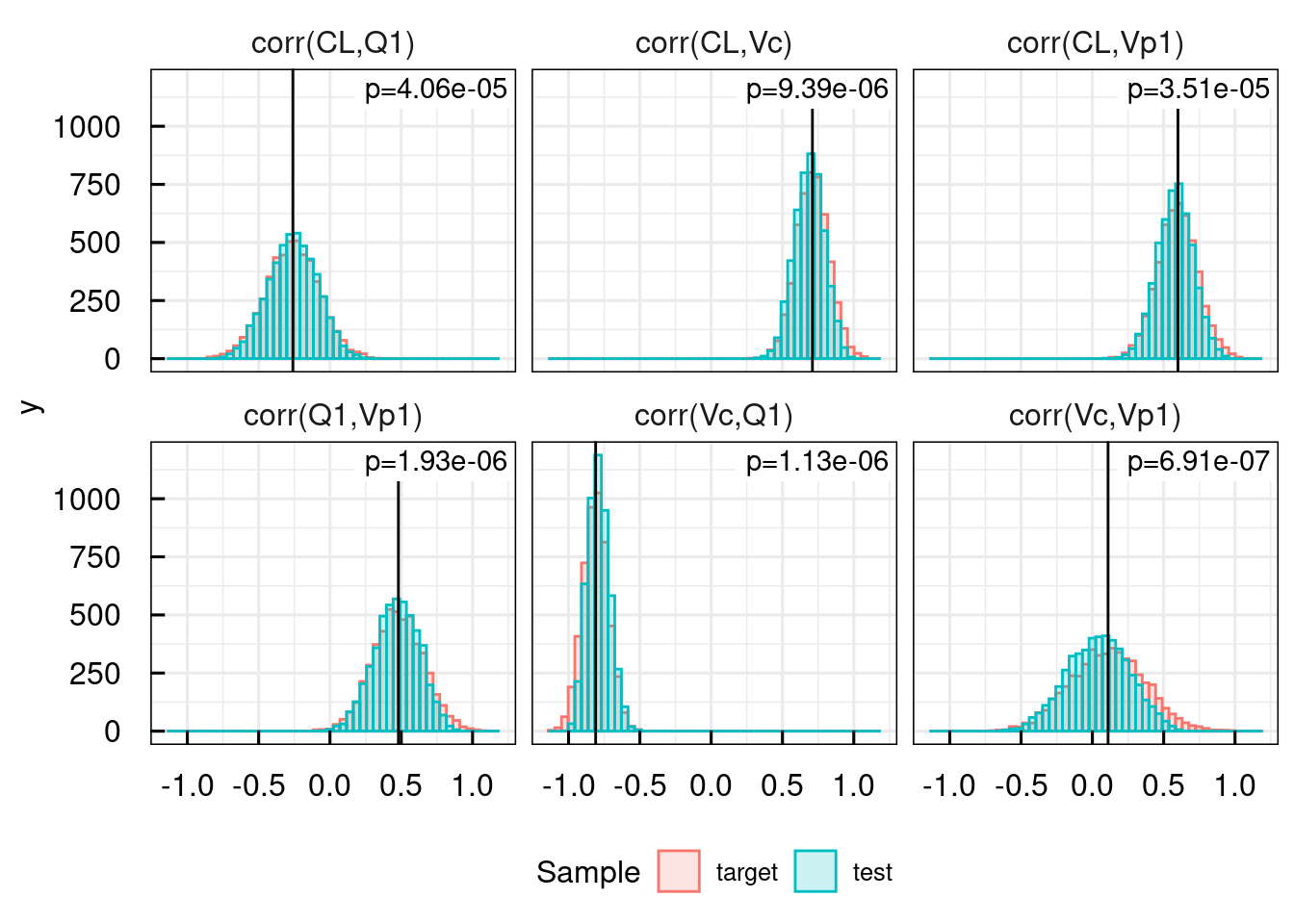
23.6.1 Detecting discrepancies in samples from the parameter uncertainty distribution
discr <- IQRtools:::detectSampleDiscrepancy(
  fileXLS <- "material/02-04-ParameterSampling/PKparameters.xlsx",
  Npop = 500, Ntests = 10)

discr$histogramsDetectedSingleParams + ggplot2::theme(legend.position = "bottom")