15 Population simulations

15.1 Basic population simulation

In pharmacometrics, population simulations are integral parts of modeling projects. On one hand they are used to check the predictiveness of the model (i.e., visual predictive checks). On the other hand simulations of virtual population support decisions, e.g., to evaluate trial designs or new, proposed posologies.

In chapter Simulation of models, we discussed the simulation of one set of parameters in combination with one dosing regimen. We show in this chapter how to efficiently simulate populations, i.e., run model simulations for multiple sets of parameters and dosing regimens. While using the same function (sim_IQRmodel()) to execute simulations as for the simple simulations, we make use of the input argument eventTable as alternative to the dosingTable and parameters. The eventTable input needs to the an IQReventTable object combining individual sets of parameters with individual dosing and potentially containing further information needed for simulation.

To give a basic overview steps to perform population simulations we go through a basic example before the customization of the simulation setup is discussed:

Basic example for population simulation using the eventTable.
Event table generation
Parameter sampling from IIV and/or parameter estimation uncertainty
Customizing population simulation by
- setting global parameters,
- setting individual simulation times

15.1.1 Basic example

The first example makes use of a base 1-compartmental PK model for theophilline that was estimated based on 12 subjects recieving a single dose of 400 mg. To perform a simulation of a population, generally, we need to define the parameters and dosing for each individual respectively.

We load the individual estimates from the model results:

# Get individual estimated parameters
indivEstimates <- getIndivParameters_IQRnlmeProject(projectPath = "material/01-07-PopulationSimulation/ExTheophilline/NONMEM")
# Get names of the parameters
paraNames <- setdiff(names(indivEstimates), c("ID", "USUBJID"))

Table 8.1: Table 8.1: Individual parameter estimates for theophilline PK
ID	ka	CL	Vc	USUBJID
1	0.0843322	2.71736	1.934910	Theo_1
2	0.0846147	2.58490	3.918930	Theo_10
3	0.0847180	4.14159	1.080320	Theo_11
4	0.0848563	2.83536	2.867530	Theo_12
5	0.0847785	3.61201	1.697320	Theo_2
6	0.0846263	3.56896	1.540070	Theo_3
7	0.0846547	3.34095	2.755240	Theo_4
8	0.0847636	2.91772	1.923560	Theo_5
9	0.0845443	4.51239	3.500380	Theo_6
10	0.0846042	3.74884	4.647100	Theo_7
11	0.0846161	3.86705	2.661180	Theo_8
12	0.0846867	4.07831	0.655227	Theo_9

We have to add the dosing information that is done using the same columns as for modeling datasets in the IQRdataGENERAL format or as used as inputs to define a dosing with IQRdosing(), i.e., by defining ID, TIME, ADM, AMT, TINF, RATE, ADDL, and II. As for modeling datasets or the IQRdosing() function, TIME, ADM and AMT are required while the others are optional and required depending on the type of dosing that is to be defined. For example, infusions need to have either the infusion time (TINF) ot the rate of infusion (RATE) defined whereas ADDL and II are superflous for single doses. As for this case all individuals receive a single dose of 400 mg theophilline at time = 0, we can simply add this information to the data frame with individual parameters:

# Add dosing information
eventData <- within(indivEstimates, {
  TIME <- 0
  ADM  <- 1
  AMT  <- 400
})

The IQReventTable is created based on the data frame eventData using the function IQReventTable() that requires to specify the names of the individual parameters that should be used in the simulation as the regression input.

# Create event table with dosing and individual parameter information
eventTable <- IQReventTable(eventData, regression = paraNames)

Table 8.3: Table 8.3: Event table to simulate individual predictions of theophilline PK
ID	ADM	AMT	TINF	ka	CL	Vc
1	1	400	1e-04	0.0843322	2.71736	1.934910
2	1	400	1e-04	0.0846147	2.58490	3.918930
3	1	400	1e-04	0.0847180	4.14159	1.080320
4	1	400	1e-04	0.0848563	2.83536	2.867530
5	1	400	1e-04	0.0847785	3.61201	1.697320
6	1	400	1e-04	0.0846263	3.56896	1.540070
7	1	400	1e-04	0.0846547	3.34095	2.755240
8	1	400	1e-04	0.0847636	2.91772	1.923560
9	1	400	1e-04	0.0845443	4.51239	3.500380
10	1	400	1e-04	0.0846042	3.74884	4.647100
11	1	400	1e-04	0.0846161	3.86705	2.661180
12	1	400	1e-04	0.0846867	4.07831	0.655227

Having the dosing and the parameters for all individuals combined in an IQReventTable object, we can use it for simulation:

# Get structural model from the NLME project
model <- IQRmodel("material/01-07-PopulationSimulation/ExTheophilline/NONMEM/model.txt")
# Load data for plotting
data <- IQRloadCSVdata("material/01-07-PopulationSimulation/ExTheophilline/data.csv")
# Define simulation tims
simtime <- seq(min(data$TIME), max(data$TIME), length.out = 201)
# Simulate
simData <- sim_IQRmodel(model, simtime, eventTable = eventTable)
# Plot individual predictions and observations
ggplot(simData, aes(TIME, OUTPUT1)) + geom_line() + facet_wrap(~ID) + geom_point(data=data, aes(y=DV), shape = 1)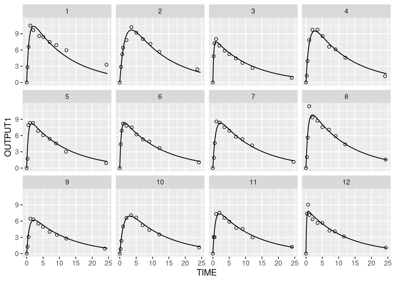

15.1.2 Event table generation

Extract dosing from dataset

dataNLME    <- IQRloadCSVdata("./material/01-07-PopulationSimulation/Ex2cptModel/data.csv")
dosing <- extract_IQRdosing(dataNLME)

dosing <- extract_IQRdosing(dataNLME, FLAGunique = TRUE, TIMEcol = "TIME")
eventDataList <- lapply(dosing, function(x) create_IQReventData(x, indivEstimates))

Individual dosing

dosing1 <- IQRdosing(TIME = 0, ADM = 1, AMT = 100, ADDL = 2, II = 24)
dosing2 <- IQRdosing(TIME = 0, ADM = 2, AMT = 50, TINF = 10)

dosing <- list(dosing1, dosing1, dosing2, dosing2)

create_IQReventData(dosing, indivEstimates[1:4,])

## Warning: List of dosings unnamed. Individuals in indivData are match by order
## of occurence.

##   TIME ADM AMT  TINF ID         ka      CL      Vc USUBJID
## 1    0   1 100 1e-04  1 0.08433216 2.71736 1.93491  Theo_1
## 2   24   1 100 1e-04  1 0.08433216 2.71736 1.93491  Theo_1
## 3   48   1 100 1e-04  1 0.08433216 2.71736 1.93491  Theo_1
## 4    0   1 100 1e-04  2 0.08461466 2.58490 3.91893 Theo_10
## 5   24   1 100 1e-04  2 0.08461466 2.58490 3.91893 Theo_10
## 6   48   1 100 1e-04  2 0.08461466 2.58490 3.91893 Theo_10
## 7    0   2  50 1e+01  3 0.08471802 4.14159 1.08032 Theo_11
## 8    0   2  50 1e+01  4 0.08485631 2.83536 2.86753 Theo_12

Time-varying parameters

dosing <- IQRdosing(TIME = 0, ADM = 1, AMT = 100, ADDL = 3, II = 24)

indivParameters <- indivEstimates[1:2,]
indivParameters$ID = 1
indivParameters$TIME = c(0,10)

create_IQReventData(dosing, indivParameters)

##   TIME ADM AMT  TINF ID         ka      CL      Vc USUBJID
## 1    0   1 100 1e-04  1 0.08433216 2.71736 1.93491  Theo_1
## 2   10  NA  NA    NA  1 0.08461466 2.58490 3.91893 Theo_10
## 3   24   1 100 1e-04  1         NA      NA      NA    <NA>
## 4   48   1 100 1e-04  1         NA      NA      NA    <NA>
## 5   72   1 100 1e-04  1         NA      NA      NA    <NA>

15.1.3 Parameter sampling

Often, models are simulated for sets of parameters sampled from an NLME model. Virtual populations are simulated based on sampled individual parameters. Or, the prediction uncertainty for a typical subject is evaluated using simulations with parameters sampled from the unceratinty distribution.

The function sample_IQRnlmeProject() is used to generate various sets of sampled individual and/or population parameters. An important input argument to this function controlling the sampling is FLAG_SAMPLE as it determines whether uncertainty, IIV, and/or covariates are considered when creating the sets of model parameters.

FLAG_SAMPLE	Sampling behavior
0	Use point estimates of population parameters (do not consider uncertainty) and sample Nsample individual patients based on these. Covariates considered if defined by user and used in model. Please note: population parameters do not take covariates into account!
1	Sample single set of population parameters from uncertainty distribution and sample Nsample individual patient parameters based on these. Covariates considered if defined by user and used in model. Please note: population parameters do not take covariates into account!
2	Sample Nsample sets of population parameters from uncertainty distribution. Do not sample from variability distribution and do not take into account covariates (even if user specified).
3	Use point estimates of population parameters (do not consider uncertainty) Return Nsamples sets of population parameters with covariates taken into account.
4	Sample single set of population parameters from uncertainty distribution Return Nsamples sets of population parameters with covariates taken into account.

Different use cases of sample_IQRnlmeProject() are illustrated in the following. The example model used is a 2-compartmental model that was build on single and multiple dose data and contains age, gender, and body weight as covariates:

# Example NLME project to illustrate parameter sampling
projectNLME <- as_IQRnlmeProject("material/01-07-PopulationSimulation/Ex2cptModel")
dataNLME    <- getData_IQRnlmeProject(projectNLME)
model <- IQRmodel("material/01-07-PopulationSimulation/Ex2cptModel/model.txt")

Virtual population

Individual parameters are sampled from an NLME project using the sample_IQRnlmeProject() function by specifying the path to the NLME project and specifying and the number of individual parameter to be returned.

# Number of individuals
Nind <- 100
# Sample individual parameters
sampleParameters <- sample_IQRnlmeProject(projectNLME, Nsamples = Nind)

## 
## No continuous covariates for sampling have been defined but the model contains the following:
## AGE0 WT0
## 
## 
## No categorical covariates for sampling have been defined but the model contains the following:
## SEX

# Outputs
sampleParameters$FLAG_SAMPLE

## [1] 0

sampleParameters$Nsamples

## [1] 100

sampleParameters$popParamValues

##           CL           Vc           ka           Q1          Vp1 
##   28.6210094   31.0098010    0.2437317   22.8036843 2324.8062961

head(sampleParameters$indParamValues)

##         CL       Vc        ka       Q1      Vp1
## 1 18.74352 16.85008 0.3663439 18.31357 5022.897
## 2 31.44678 31.65958 0.2333856 35.15699 2244.054
## 3 13.09969 23.22566 0.4809457 14.99012 1945.770
## 4 21.42965 34.38950 0.2832930 25.82940 1477.804
## 5 48.45593 28.36028 0.1770285 18.40066 2961.775
## 6 34.22848 39.38761 0.3652917 32.94980 1782.496

The function returns information about the sampling (FLAG_SAMPLE and Nsamples), population parameters (popParamValues) and individual parameters (indParamValues). For default, the function does not consider uncertainty (FLAG_SAMPLE = 0), thus the virtual population is based on the point estimates of the model parameters.

To sample with considering covariates, the input argument covariates is used which can a data frame or matrix with individual information per row and named columns containing the covariate values. Note that the function return a data frame of individual parameter including also the subject ID which is later needed to create an event table for simulation.

# Define covariates for individuals
covariates <- data.frame(
  ID = 1:Nind,
  SEX = sample(c(1,2), Nind, replace = TRUE),
  AGE0 = runif(Nind, min=20, max = 65),
  WT0 = runif(Nind, min = 45, max = 100)
)
# Sample individual parameters while considering covariate information
indivParameters <- sample_IQRnlmeProject(projectNLME, covariates = covariates, FLAGid = TRUE)$indParamValues
# Visualize covariates dependency of parameters
x <- merge(covariates, indivParameters, by = "ID")
p1 <- ggplot(x, aes(WT0, ka)) + geom_point() + geom_smooth() + scale_y_log10()
p2 <- ggplot(x, aes(AGE0, ka)) + geom_point() + geom_smooth() + scale_y_log10()
p3 <- ggplot(x, aes(as.factor(SEX), CL)) + geom_boxplot() + scale_y_log10()
gridExtra::grid.arrange(p1,p2,p3, nrow = 1)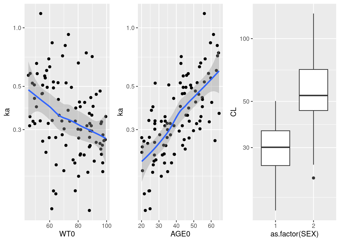

Virtual populations considering estimation uncertainty

To simulate population while also accounting for parameter estimation uncertainty, we need to set FLAG_SAMPLE = 1. Several populations are created for which new population-level parameters (fixed effects and distribution of IIVs) are sampled from the parameter covariance matrix:

# Number of populations
Npop <- 100
# Sample individual parameters for each population
sampleParametersPop <- lapply(1:Npop, function(k) 
  sample_IQRnlmeProject(projectNLME, FLAG_SAMPLE = 1, covariates = covariates, FLAGid = TRUE)
)
names(sampleParametersPop) <- 1:Npop
# Collect individual parameters into data frame
indivParametersPop <- plyr::ldply(sampleParametersPop, function(x) x$indParamValues, .id = "IDpop")
indivParametersPop$IDpop <- as.numeric(indivParametersPop$IDpop)
indivParametersPop$ID <- indivParametersPop$ID + Nind*10 * (indivParametersPop$IDpop-1)
# Collect population parameters into data frame
popParametersPop <- plyr::ldply(sampleParametersPop, function(x) x$popParamValues, .id = "IDpop")
popParametersPop$IDpop <- as.numeric(popParametersPop$IDpop)

ggplot(indivParametersPop, aes(IDpop, CL)) + geom_point(shape=1, alpha= 0.3) +
  geom_point(data=popParametersPop, color = "firebrick") + scale_y_log10()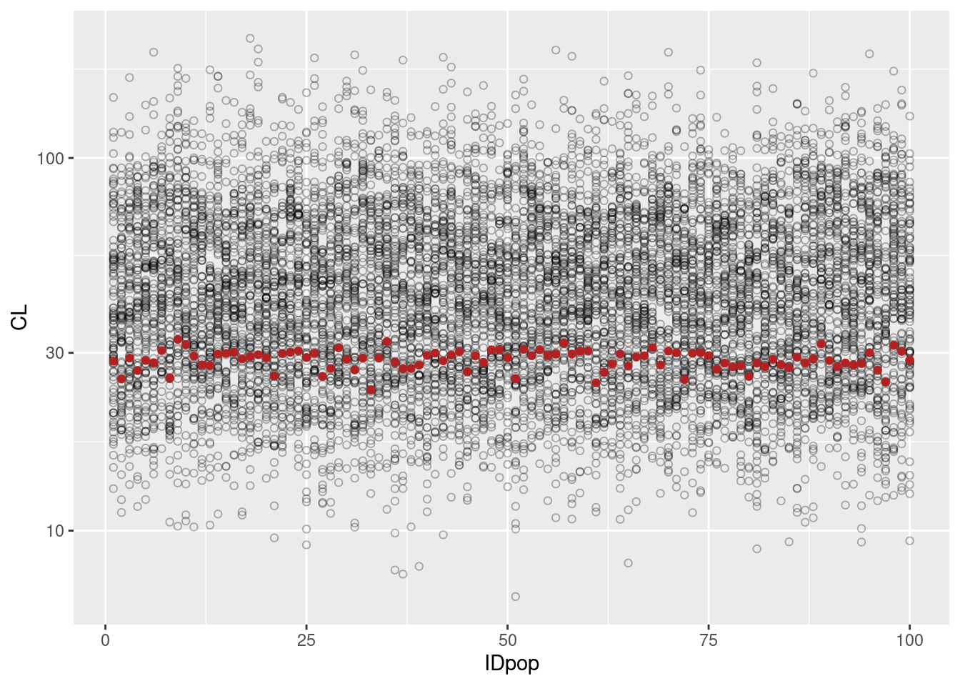

Prediction uncertainty for typical subject

The prediction uncertainty is assessed when sampling only from the uncertainty of the estimated parameter distribution.

# Sample parameters
popParameters <- sample_IQRnlmeProject(projectNLME, Nsamples = 100, FLAG_SAMPLE = 2, FLAGid = TRUE)$popParamValues
# Add dosing
eventData <- create_IQReventData(IQRdosing(TIME = 0, ADM = 1, AMT = 100), popParameters)
# Create event table
eventTable <- IQReventTable(eventData, regression = setdiff(names(popParameters),"ID"))
# Simulate
simUncertainty <- sim_IQRmodel(model, simtime = seq(0.2,80, by = 0.2), eventTable = eventTable, FLAGoutputsOnly = TRUE)
# Plot predictions and confidence interval
ggplot(simUncertainty, aes(TIME,OUTPUT1)) + scale_y_log10()+
  stat_summary(fun.data = median_hilow, geom = "ribbon", alpha = 0.3) +
  stat_summary(fun.data = median_hilow, geom = "line") +
  ggtitle("Simulation of reference subject with 95%-CI")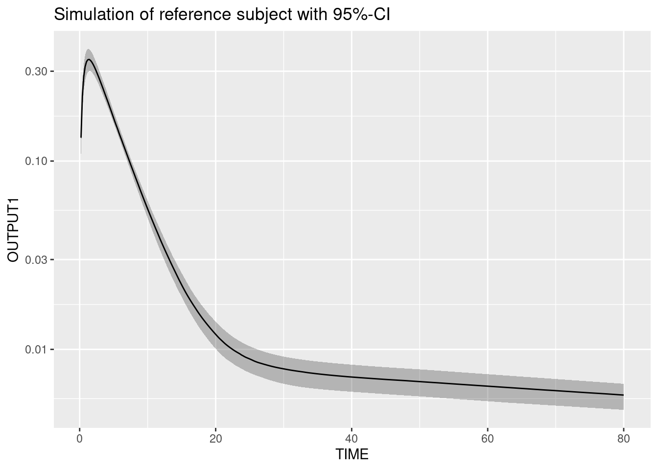

Prediction differences due to covariates

Prediction differences exclusively due to covariate characteristics can be assessed using the FLAG_SAMPLE = 3. Here, we show differences betwenn the male and the female subpopulations.

# Sample parameters
popParameters <- sample_IQRnlmeProject(projectNLME, covariates = covariates, FLAG_SAMPLE = 3, FLAGid = TRUE)$popParamValues
# Add dosing
eventData <- create_IQReventData(IQRdosing(TIME = 0, ADM = 1, AMT = 100), popParameters)
# Create event table
eventTable <- IQReventTable(eventData, regression = setdiff(names(popParameters),"ID"))
# Simulate
simCovDifference <- sim_IQRmodel(model, simtime = seq(0.2,80, by = 0.2), eventTable = eventTable, FLAGoutputsOnly = TRUE)
# Plot predictions and confidence interval
simCovDifference <- merge(simCovDifference, covariates, by = "ID")
simCovDifference$SEX <- factor(simCovDifference$SEX, levels = c(1,2), labels = c("male", "female"))
ggplot(simCovDifference, aes(TIME,OUTPUT1, color = SEX, fill = SEX, group = SEX)) +
  stat_summary(fun.data = median_hilow, geom = "ribbon", alpha = 0.3) +
  stat_summary(fun.data = median_hilow, geom = "line") +
  scale_y_log10() + scale_color_manual(values = c("darkorange", "olivedrab")) + scale_fill_manual(values = c("darkorange", "olivedrab")) +
  ggtitle("Differences for female and male subpopulation considering covariates, but no IIV")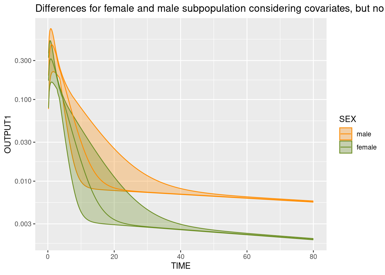

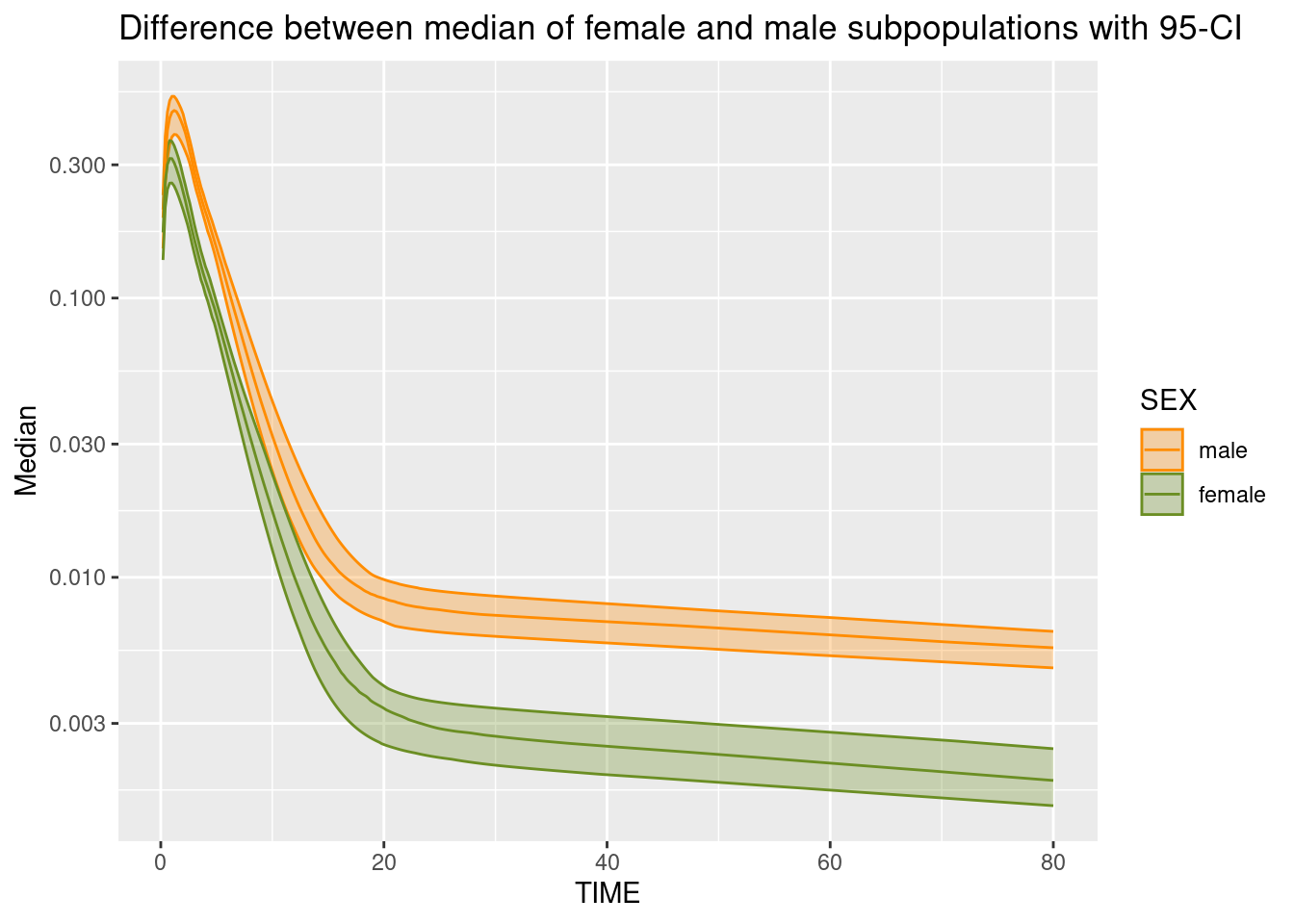
Predictions for covariate differences with uncertainty