9 Model definition

IQR Tools implements a general and powerful ODE and biochemical reaction expression based model description language, allowing to describe most models used in systems biology, systems pharmacology, and pharmacometrics. Tools are available to support the development, manipulation, and simulation of models.

9.1 Model definition basics

9.1.1 Biochemical reaction model

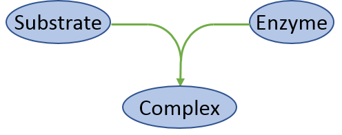
The basics of model representation in IQR Tools is illustrated for a model describing the (irreversible) formation of a complex C between a substrate A and an enzyme B (see Figure below). These types of processes are common as motifs in larger models of signaling pathways.

In IQR Tools models are described in txt-files containing different sections for the different elements (e.g., states, parameters, etc.) of the model. Some of the sections may be empty. MODEL FUNCTIONS and MODEL EVENTS for example are used for representation of more complex models which is explained in Section Advanced model representation. The txt-file of the model takes the following form:

********** MODEL NAME
Biochemical reaction model 
********** MODEL NOTES
Concentration changes due to biochemical reaction given as differential equations
********** MODEL STATES
d/dt(Substrate) = -R1
d/dt(Enzyme)    = -R1
d/dt(Complex)   =  R1

Substrate(0) = 1
Enzyme(0)    = 1
Complex(0)   = 0
********** MODEL PARAMETERS
k1 = 0.5
********** MODEL VARIABLES

********** MODEL REACTIONS
R1 = k1 * Substrate * Enzyme
********** MODEL FUNCTIONS

********** MODEL EVENTS

The MODEL STATES section contains the ordinary differential equations that define the changes of each state with time and their initial value at t=0. Initial state values may be omitted if they are 0. Another feature is that an initial state does not need to be a numerical value but could also be a model parameter.

The reaction rate for this binding reaction is defined in the MODEL REACTIONS section. It could be defined directly in the state equations, but this may be confusing for more complex reaction networks.

Having defined the model in a text file, it can be loaded, simulated, and the simulation results visualized with IQR Tools. The chapter Basic simulation of models illustrates how to simulate models with IQR tools in more detail.

# load model
filename <- "material/01-02-ModelImplementation/model_Example1.txt"
model <- IQRmodel(filename)

# simulate the model for 100 time units
sim_results <- sim_IQRmodel(model,100)   

# plot the simulation results for the complex
plot(sim_results)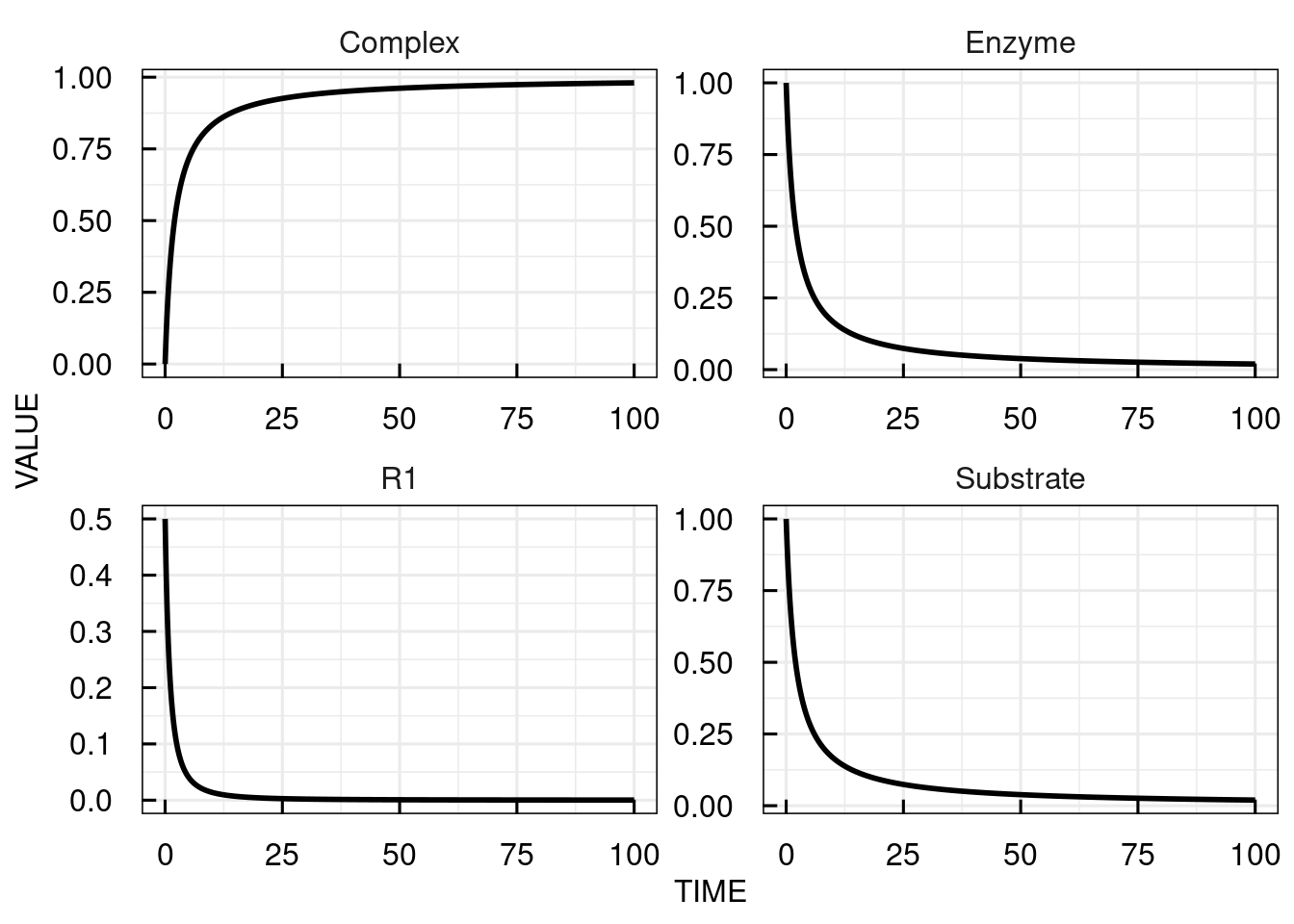

Alternatively to the differential equations, a representation can be used that resembles the common syntax for writing (bio-)chemical reactions.

********** MODEL NAME
Biochemical reaction model

********** MODEL NOTES
Biochemical reaction representation
********** MODEL STATE INFORMATION
Substrate(0) = 1
Enzyme(0)    = 1
Complex(0)   = 0
********** MODEL PARAMETERS
k1 = 0.5
********** MODEL VARIABLES

********** MODEL REACTIONS
Substrate + Enzyme  => Complex  :  R1
    vf = kon * Drug * Target
********** MODEL FUNCTIONS
********** MODEL EVENTS

Here, the MODEL STATES section was substituted by the MODEL STATE INFORMATION section, containing only the initial state values. In the MODEL REACTIONS section, the reaction equation is given followed by its name (R1) after a colon. The (forward) rate (vf) is defined below.

In this representation it is easy to switch the reaction to be reversible by adjusting the arrow type and giving the rate for the reverse reaction:

********** MODEL REACTIONS
Substrate + Enzyme  <=> Complex  :  R1
    vf = kon * Drug * Target
    vr = koff * Complex

9.1.2 One compartment linear PK

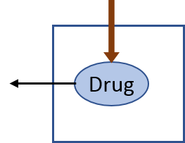
A one-compartment linear pharmacokinetic model with an initial single dose can be implented in IQR Tools as follows:

********** MODEL NAME
Linear 1-compartmental PK model
********** MODEL NOTES
Linear 1-compartmental PK model with initial single dose
********** MODEL STATES
d/dt(Ac) = -CL/Vc*Ac
Ac(0) = Dose 
********** MODEL PARAMETERS
CL    =  20    # (L/hour)   Clearance
Vc    =  32    # (L)         Central volume
Dose  = 100    # (mg)       Dose
********** MODEL VARIABLES
Cc = Ac/Vc * 1000     # (ng/mL) Plasma concentration
********** MODEL REACTIONS
********** MODEL FUNCTIONS
********** MODEL EVENTS

The MODEL VARIABLES section is here used to define the plasma concentration based on the amount (a state) and the central volume (a parameter). Variables could also be used in the definiton of the ODEs in the MODEL STATES section or in the MODEL REACTIONS section.

# load model
filename <- "material/01-02-ModelImplementation/model_Example2.txt"
model <- IQRmodel(filename)

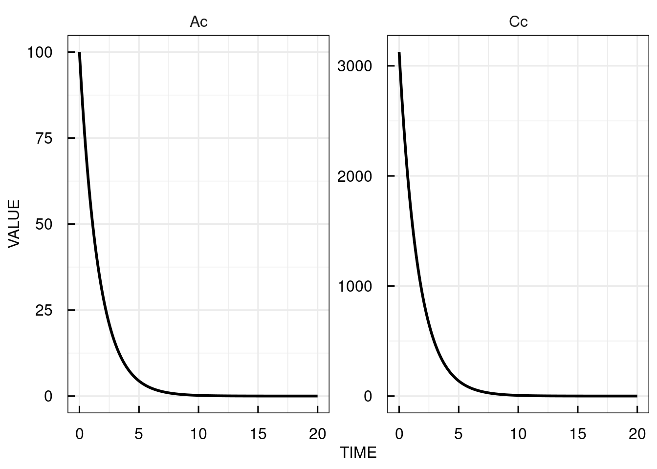
# simulate model for 20 hours
sim_results <- sim_IQRmodel(model,20)    

# plot the simulated plasma concentration
plot(sim_results)

9.1.3 PK/PD

ODEs and biochemical reactions can be used simultaneously. As an example, the pharmacokinetic model is linked with a binding reaction to a clinical response.

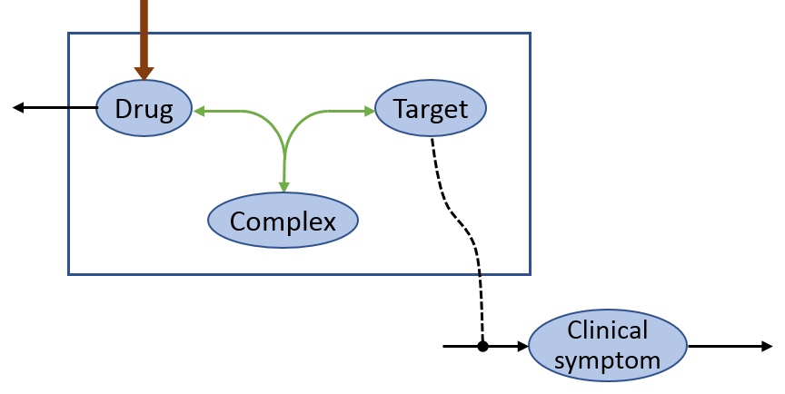
The PK and the changes of the clinical symptoms in dependency of a target molecule are coded with differential equations whereas the binding reaction of the drug to the target molecule is defined as a biochemical reaction.

********** MODEL NAME
Drug target binding with indirect clinical response
********** MODEL NOTES
Target indirectly stimulating clinical symptoms.
Drug binds to target forming a non-stimulating complex.
********** MODEL STATE INFORMATION
d/dt(Ac)            = -CL/Vc*Ac
d/dt(ClinSym)       = rinS - koutS * ClinSym
Ac(0)               =  Dose
ClinSym(0)          =  ClinSymBase
Target(0)           =  TargetBase
********** MODEL PARAMETERS
# PK
CL          =  20       # (L/hour)   Clearance
Vc          =  32       # (L)        Central volume
Dose        =  10       # (mg)       Dose
MW          = 400       # (g/mol)    Molecular weight
TargetBase  =   3       # (nM)       Baseline target levels
ClinSymBase = 100       # (score)    Clinical symptom score at baseline
koutS       =   0.2     # (-)        Turnover rate of clinical symptoms
KD          =  50       # (nM)       Binding dissociation constant
koff        =   0.1     # (1/h)      Dissociation rate constant
********** MODEL VARIABLES
Cc        = Ac/Vc * 1000                     # (ng/mL) plasma concentration
Stim      = ClinSymBase/TargetBase * koutS   # clinical symptom stimulation factor
rinS      = Stim * Target                    # symptom input rate
kon       = koff/KD                          # binding rate constant
********** MODEL REACTIONS
# Reversible binding reaction
Cc + Target  <=> Complex  :  Rbind
    vf = kon * Cc/MW*1000 * Target
    vr = koff * Complex
********** MODEL FUNCTIONS
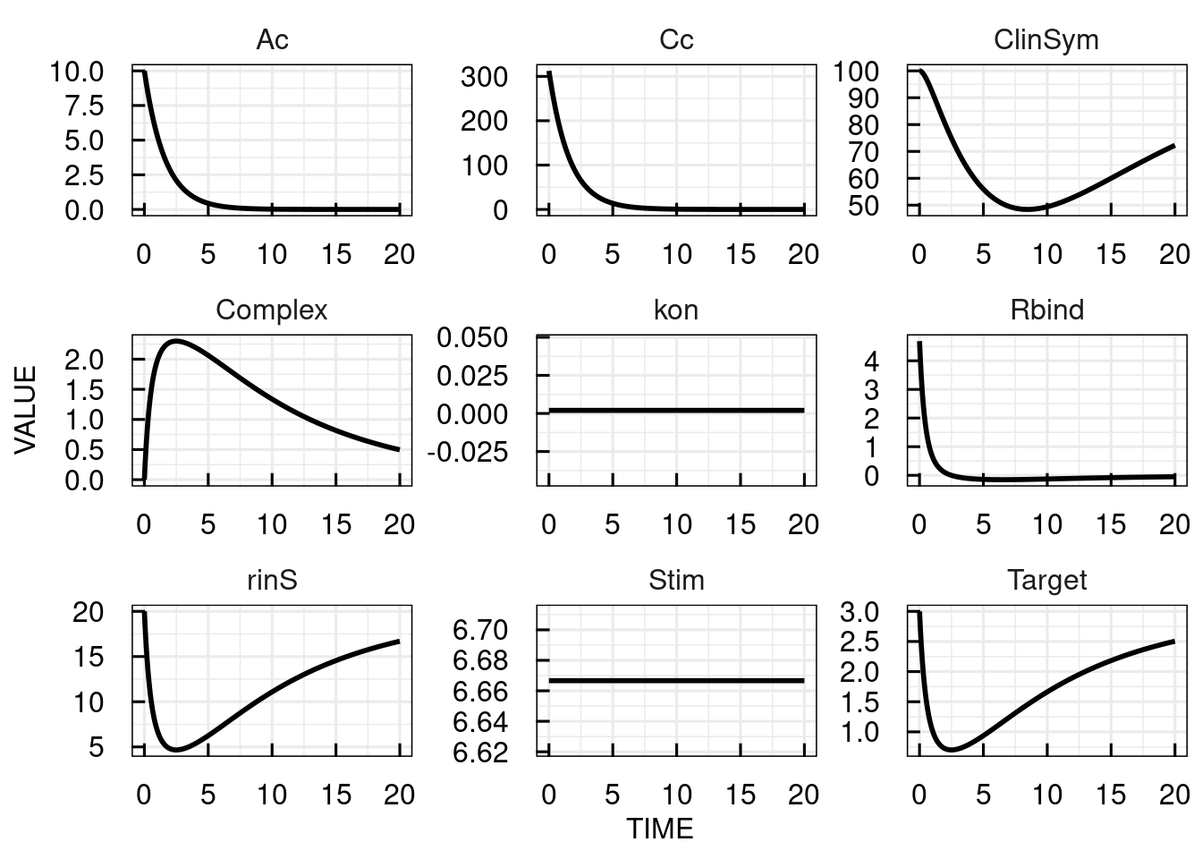
********** MODEL EVENTS

The PK, free target molecule levels and clinical symptoms are simulated in IQR Tools:

9.2 Dosing representation

Usually, pharmacokinetic models need to handle different and complex dosing regimens. An implementation directly in the model as shown in the PK model example above is not sufficient for more complex regimens or other tasks than simulation. Instead, the PK model and the dosing are separated. In the model, a variable INPUT1 is added to the compartment (amount of drug) to which the dose is administered.

********** MODEL NAME
Linear 1-compartmental PK model
********** MODEL NOTES
Linear 1-compartmental PK model with initial single dose
********** MODEL STATES
d/dt(Ac) = -CL/Vc*Ac    + INPUT1
Ac(0) = 0 
********** MODEL PARAMETERS
CL    =  20    # (L/hour)   Clearance
Vc    =  32    # (L)         Central volume
********** MODEL VARIABLES
Cc = Ac/Vc * 1000     # (ng/mL) Plasma concentration
********** MODEL REACTIONS
********** MODEL FUNCTIONS
********** MODEL EVENTS

The dosing is defined by the function IQRdosing() with (at least) defining the time of dosing (“TIME”), the dose amount (“AMT”) and the input number (“ADM”) as there can be more input variables present. This way it is easy to simulate the PK model with two bolus inputs of 10 mg at time 0 and 10.

# load model
filename <- "material/01-02-ModelImplementation/model_Example4.txt"
model <- IQRmodel(filename)

# define the dosing scheme
dosing <- IQRdosing(TIME=c(0,10),ADM=c(1,1),AMT=c(10,10))

# simulate model for 20 time units
sim_results <- sim_IQRmodel(model,20,dosingTable=dosing)     

# plot the simulation results for the central compartment
plot(sim_results)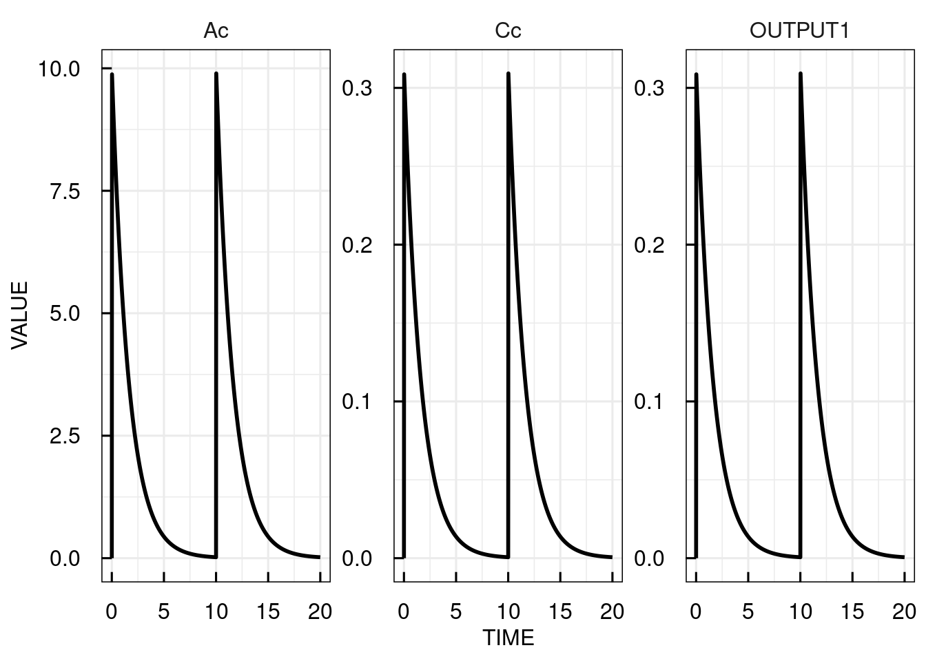

Infusions (and zero-order absorption after oral dosing) are implemented by defing a rate (RATE) of infusion or the infusion duration (TINF). First order absorption would be coded in the model with a bolus administration to an additional dosing compartment. For any dosing event, the parameter “LAGTIME” can specify a lag time before the dosing.

9.3 Advanced model definition

9.3.1 Example

Assume a drug which basically has a 1-compartmental PK as in the example above, but a limited clearance and parameters changing with time and impacted by the dosing. A PD effect (PD) is directly linked to the plasma concentration (c).

To implement this model, (advanced) model syntax is used. Conditional statements are defined for modulation of the absorption rate constant. Model events are used to define when the last dose was given. Interpolation function is used to define the time-varying Michaelis-Menten constant. The Michealis-Menten equation is a user-defined function.

An implementation of the model as an IQR model is:

********** MODEL NAME
Advanced PK model
********** MODEL NOTES
1-compartmentl PK model with ka doubled in the first 30 min after dosing and a Michaelis-Menten like limitation on clearance that increases with time.
Assume time in hours.
********** MODEL STATES
# PK model
d/dt(Ad) = -kaINST*Ad           + INPUT1
d/dt(Ac) =  kaINST*Ad - CLinst
# dummy state indicating when to apply increased KA
d/dt(DUMMY1) = INPUT1
# dummy state indicating whether first dose was already given
d/dt(DUMMY2) = INPUT1
# count time after dose only when first dose was already given
d/dt(timeAfterDose) = flag
Ad(0) = 0
Ac(0) = 0
********** MODEL PARAMETERS
ka = 0.6
CL = 20
Vc = 12
********** MODEL VARIABLES
# Set instantaneous KA based on dummy state 1
#  (DUMMY1 is not empty)
kaINST = piecewise(ka,eq(DUMMY1,0),2*ka)

# Set flag if first dose was already given
#  (DUMMY2 is not empty)
flag = piecewise(0,eq(DUMMY2,0),1)

# Time varying Michaelis-Menten constant
kM = interp1([0,12,24],[0.1,1,10],time)

# Plasma concentration
Cc = Ac/Vc

# PD effects
PD = log(Cc)^2
********** MODEL REACTIONS
CLinst = CL/Vc * MM_function(Cc,kM)
********** MODEL FUNCTIONS
# Define Michaelis-Menten function
MM_function(x,kA) = x/(x+kA)
********** MODEL EVENTS
# Reset time after dose to 0 when dosing occurs
Event1 = gt(DUMMY1,0),timeAfterDose,0

# Empty dummy state after 0.5 hours
Event2 = gt(timeAfterDose,0.5),DUMMY1,0

These are the simulated timecourses for 5 doses of 10 mg each 12 hours:

# load model
filename <- "material/01-02-ModelImplementation/model_Example5.txt"
model <- IQRmodel(filename)

# define the dosing scheme
dosing <- IQRdosing(TIME=seq(0,48,by=12),ADM=rep(1,5),AMT=rep(10,5))

# simulate model for 20 time units
sim_results <- sim_IQRmodel(model,72,dosingTable=dosing)     

# plot the simulation results for the central compartment
plot(sim_results)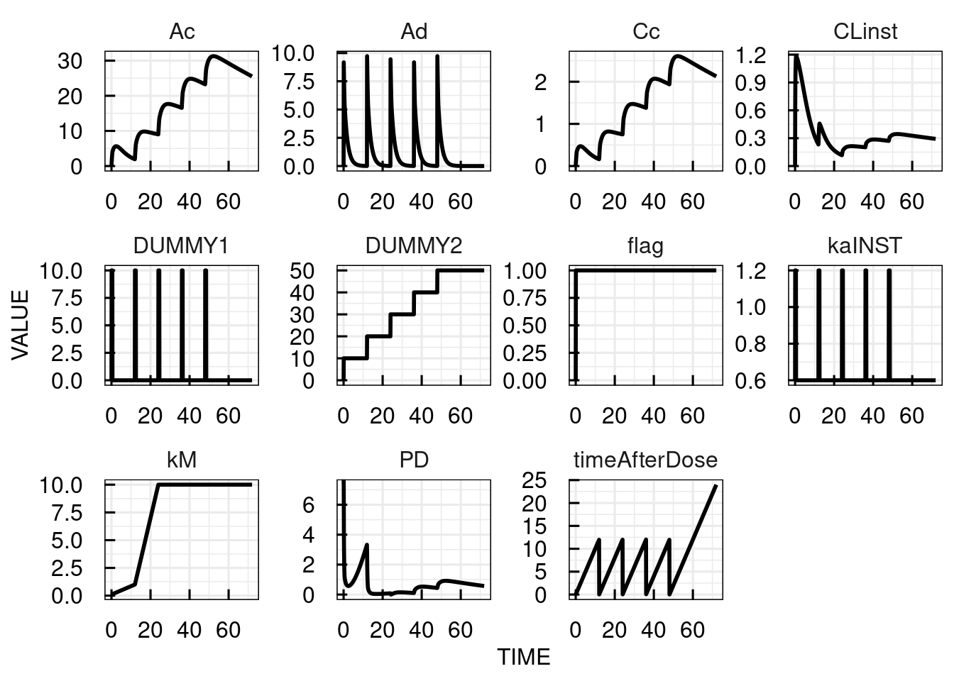

In the following, the different parts of the model description above are discussed in detail. For general information about the parts of the model description, please refer to the model section descripton in the technical details.

9.3.2 Lagtimes

Whenever an INPUT* is defined in a model (where “*” is the number of the input) then a parameter Tlag*, which represents the lagtime for this input, is assumed to be present in the model. The user can code this parameter manually in the text representation of the model, or if this parameter is not present, then it is added automatically upon import of a text representation, and initialized with 0.

9.3.3 Mathematical functions

Basic mathematical functions, i.e., the natural logarithm (“log”) and power (“^”), are needed for linking the the plasma concentrations to the PD effect. Many other basic mathematical functions are available with an intuitive notation. Most commonly used are

• log (natural logarithms)
• exp (natural exponential function)
• min (minimum)
• max (maximum)
• sqrt (square root)
• ^ (power operator)

Please refer to the section Pre-defined functions for a complete list.

9.3.4 Implementing conditional statements (if-then-else)

In the model in section Advanced model representation the absorption rate value used in the ODE is high if the last dose was given less than 30 min ago and low otherwise. This is a conditional statements (if-then-else) that is implemented in IQRtool via the “piecewise” function:

# Set instantaneous KA based on dummy state 1
#  (DUMMY1 is not empty)
kaINST = piecewise(ka,eq(DUMMY1,0),2*ka)

Here, DUMMY1 indicates the time after dose until 30 min (DUMMY1 is 1 for 0-30 min after the last dose and 0 otherwise). The second argument checks whether DUMMY1 is 0. If this is true, the first argument (ka) is returned, the third argument (2*ka) otherwise.

Conditional statements use value comparisons (e.g., “a is less than b”, “c is equal to b”) and Boolean operators (AND, OR, etc. ) as also shown in the example above which are implemented using the IQR Tools function in the following table:

Comparison/Operator	IQR Tools function
<	lt
>	gt
<=	le
>=	ge
=	eq
AND	and
OR	or

9.3.5 Interpolation functions

In the model in section Advanced model representation the Michaelis-Menten constant is linearily interpolated from 0.1 to 1 and 1 to 10 between time points 0 and 12 hours, and 12 and 24 hours. The first argument to the interpolation function “interp1” defines the time points and the second which values kM should assume at these timepoints. The third argument indicates the variable specifying the current time point.

# Time varying Michaelis-Menton constant
kM = interp1([0,12,24],[0.1,1,10],time)

The table below lists the interpolation functions available in IQR tools:

Function	Description
interp0	Zero order interpolation (constant values between support points)
interp1	First order (linear) interpolation
interpcs	Cubic spline interpolation

9.3.6 MODEL FUNCTIONS section

The user can also define own functions that can be used in the other model sections. In the example in section Advanced model representation, the Michaelis-Menten equation was defined as a function such that could be called by its name in the MODEL REACTIONS section:

********** MODEL REACTIONS
CLinst = CL/Vc * MM_function(Cc,kM)

********** MODEL FUNCTIONS
# Define Michaelis-Menten function
MM_function(x,kA) = x/(x+kA)

Definition of functions can be useful for improving readability in case of complicated expressions or terms that are repeatedly used in the model.

9.3.7 MODEL EVENTS section

In the model in section Advanced model representation, the state “DUMMY1” is an indicator of whether the last dosing time point was no more than 30 min ago or not. It is recognizing a dose as the INPUT1 is added to this state and DUMMY1 is no longer empty after a dose. However, it is reset to 0 at 0.5h so that it can be changed also for later doses. At the same time, the state “timeafterdose” which is increasing along with time needs to be reset to zero if a dose is given, i.e., when DUMMY1 is not empty anymore.

In the IQR model representation, instant changes of states (or variables) are implemented using model events:

********** MODEL EVENTS
# Reset time after dose to 0 when dosing occurs
Event1 = gt(DUMMY1,0),timeAfterDose,0

# Empty dummy state after 0.5 hours
Event2 = gt(timeAfterDose,0.5),DUMMY1,0

An event statement consists of a condition when the event occurs followed by the name of the state to be changed and the value to which it is reset. The “Event1” in the example reads: if “DUMMY1” becomes greater than 0, set “timeafterdose” to 0.

9.4 Handling of models in R

9.4.1 Model import

An example of how to import an existing model using the function IQRmodel() is shown below. The extension of the model file name is arbitrary. It is suggested to use “.txt” for ODE based models, and “.txtbc” for models in the biochemical representation. But other extensions can be used if desired.

When importing a model an object of class “IQRmodel” is created.

# Load existing model
filename <- "material/01-02-ModelImplementation/model_Example1.txt"
model <- IQRmodel(filename)

# Inspect class of created object
class(model)

## [1] "IQRmodel"

9.4.2 Support of SBML

Systems Pharmacology gains in interest in the Modeling and Simulation community. Thus does also the Systems Biology Markup Language (SBML), in which many systems pharmacology type of models are coded (see, e.g. Biomodels Database).

SBML, however, is very badly supported when using R. Some packages (such as SBMLR) are available and claim to be able to import and simulate SBML models. However, typically, not all features of SBML models are considered.

In order to allow IQR Tools to import SBML models a workaround needed to be found. This workaround comes in the form of the IQRsbml software that needs to be installed separately on the computer.

Once installed, the path to the executable needs to be provided in the setup of IQR Tools (see Section ??. After that IQR Tools can easily import SBML models (Level 2 Version 1,2,3,4) as IQRmodels with the following command:

modelSBML <- IQRmodel("sbmlModelFile.xml")

IQRsbml is only provided for Windows 64 bit systems.

9.4.3 Basic model information

Basic information about the model is displayed when calling the model variable. The IQRmodel object stores the definitions given in the model sections and some further elements as list elements that can be accessed using the $-operator. Further information is stored as attributes which are described in the model attributes section in the model definition chapter.

# Display basic model information
model

##  IQRmodel
##  ========
##  Name:                       Biochemical reaction model 
##  Number States:              3 
##  Number Parameters:          1 
##  Number Variables:           0 
##  Number Reactions:           1 
##  Number Functions:           0 
##  Number Events:              0 
##  Number Inputs:              0 
##  Number Outputs:             0

# Names of model sections/elements
names(model)

## [1] "name"       "notes"      "parameters" "states"     "reactions"

# Access a model section, e.g., the model parameters
model$parameters

## $k1
## $k1$value
## [1] 0.5
## 
## $k1$type
## NULL
## 
## $k1$compartment
## NULL
## 
## $k1$unittype
## NULL
## 
## $k1$notes
## NULL

9.4.4 Model export

To export a model to a txt file we use the export_IQRmodel() function. In the following example the model is saved in txt file called “model.txt” in the current working directory. The model can also be exported in the biochemical reaction representation by setting “FLAGbc = TRUE”. The export function can also be used to view the model on the console during working.

# export an existing model
filename <- file.path(getwd(),"model.txt")
export_IQRmodel(model,filename)

# View the exported model on the console
cat(export_IQRmodel(model))

## ********** MODEL NAME
## 
## Biochemical reaction model
## 
## ********** MODEL NOTES
## 
## Concentration changes due to biochemical reaction given as differential equations
## 
## ********** MODEL STATES
## 
## d/dt(Substrate) = -R1
## d/dt(Enzyme) = -R1
## d/dt(Complex) = R1
##  
## Substrate(0) = 1
## Enzyme(0) = 1
## Complex(0) = 0
##  
## ********** MODEL PARAMETERS
## 
## k1 = 0.5
##  
## ********** MODEL VARIABLES
## 
##  
## ********** MODEL REACTIONS
## 
## R1 = k1 * Substrate * Enzyme
##  
## ********** MODEL FUNCTIONS
## 
##  
## ********** MODEL EVENTS
## 
##  
## ********** MODEL INITIAL ASSIGNMENTS
## 
## 

# View the exported model as biochemical reactions on the console
cat(export_IQRmodel(model, FLAGbc = TRUE))

## For export in BC notation the underlying assumptions are:

##   * All reaction rates are defined in amount/time units

##   * Species ideally in amount and ODEs defined by sum of reaction rates

##     * Stoichiometric factors can be numeric or parameters and need to be define in front of reaction names

##       Example: d/dt(speciesAmount) = 2*reaction1 - reaction2 - 1*reaction3

## ********** MODEL NAME
## 
## Biochemical reaction model
## 
## ********** MODEL NOTES
## 
## Concentration changes due to biochemical reaction given as differential equations
## 
## ********** MODEL STATE INFORMATION
## 
##  
## Substrate(0) = 1
## Enzyme(0) = 1
## Complex(0) = 0
##  
## ********** MODEL PARAMETERS
## 
## k1 = 0.5
##  
## ********** MODEL VARIABLES
## 
##  
## ********** MODEL REACTIONS
## 
## Substrate+Enzyme => Complex : R1
##  vf = k1 * Substrate * Enzyme
## 
## ********** MODEL FUNCTIONS
## 
##  
## ********** MODEL EVENTS
## 
##  
## ********** MODEL INITIAL ASSIGNMENTS
## 
## 

9.5 PK model library

A PK model library is available in the documentation material: material/ModelLibraryPK.

9.6 Example models

In this section some model definitions for certain models are shown.

9.6.1 PBPK

********** MODEL NAME
Example PBPK model
********** MODEL NOTES
Dose: mg
Concentrations: ng/mL
Time: hours
********** MODEL STATES
# Differential equations, implementing a PBPK model
d/dt(Lungs)          = QLU*(Venous_Blood/VVB - Lungs/KbLU/VLU)
d/dt(Heart)          = QHT*(Arterial_Blood/VAB - Heart/KbHT/VHT)
d/dt(Brain)          = QBR*(Arterial_Blood/VAB - Brain/KbBR/VBR)
d/dt(Muscles)        = QMU*(Arterial_Blood/VAB - Muscles/KbMU/VMU)
d/dt(Adipose)        = QAD*(Arterial_Blood/VAB - Adipose/KbAD/VAD)
d/dt(Skin)           = QSK*(Arterial_Blood/VAB - Skin/KbSK/VSK)
d/dt(Spleen)         = QSP*(Arterial_Blood/VAB - Spleen/KbSP/VSP)
d/dt(Pancreas)       = QPA*(Arterial_Blood/VAB - Pancreas/KbPA/VPA)
d/dt(Liver)          = QHA*Arterial_Blood/VAB + QSP*Spleen/KbSP/VSP + QPA*Pancreas/KbPA/VPA + QST*Stomach/KbST/VST + QGU*Gut/KbGU/VGU - CLint*fub*Liver/KbLI/VLI - QLI*Liver/KbLI/VLI
d/dt(Stomach)        = QST*(Arterial_Blood/VAB - Stomach/KbST/VST)
d/dt(Gut)            = QGU*(Arterial_Blood/VAB - Gut/KbGU/VGU)
d/dt(Bones)          = QBO*(Arterial_Blood/VAB - Bones/KbBO/VBO)
d/dt(Kidneys)        = QKI*(Arterial_Blood/VAB - Kidneys/KbKI/VKI)
d/dt(Arterial_Blood) = QLU*(Lungs/KbLU/VLU - Arterial_Blood/VAB)
d/dt(Venous_Blood)   = QHT*Heart/KbHT/VHT + QBR*Brain/KbBR/VBR + QMU*Muscles/KbMU/VMU + QAD*Adipose/KbAD/VAD + QSK*Skin/KbSK/VSK + QLI*Liver/KbLI/VLI + QBO*Bones/KbBO/VBO + QKI*Kidneys/KbKI/VKI + QRB*Rest_of_Body/KbRB/VRB - QLU*Venous_Blood/VVB + INPUT1
d/dt(Rest_of_Body)   = QRB*(Arterial_Blood/VAB - Rest_of_Body/KbRB/VRB)

********** MODEL PARAMETERS
# Define some parameters
# These are the ones that are estimated in the example
CLint   = 1998.196  # Intrinsic clearance
KbBR    = 3.004166  # Partition coefficient - Brain
KbMU    = 1.349859  # Partition coefficient - Muscle
KbAD    = 7.389056  # Partition coefficient - Adipose
KbBO    = 1.030455  # Partition coefficient - Bone
KbRB    = 1.349859  # Partition coefficient - Rest of body

# Define some additional parameters
BP      = 0.61     # Blood:plasma partition coefficient
fup     = 0.028    # Fraction unbound in plasma

# Define additional partition coefficients
KbLU    = 2.301129
KbHT    = 3.066387
KbSK    = 0.5922657
KbSP    = 1.380437
KbPA    = 1.380437
KbLI    = 5.814763
KbST    = 1.380437
KbGU    = 3.32876
KbKI    = 3.732581

# Define regression parameters
WT      = 70
********** MODEL VARIABLES
# Determine fraction unbound in blood
fub     = fup/BP

# Define regional blood flows
CO      = (187.00*WT^0.81)*60/1000 # Cardiac output (L/h) from White et al (1968)
QHT     = 4.0 *CO/100
QBR     = 12.0*CO/100
QMU     = 17.0*CO/100
QAD     = 5.0 *CO/100
QSK     = 5.0 *CO/100
QSP     = 3.0 *CO/100
QPA     = 1.0 *CO/100
QLI     = 25.5*CO/100
QST     = 1.0 *CO/100
QGU     = 14.0*CO/100
QHA     = QLI - (QSP + QPA + QST + QGU) # Hepatic artery blood flow
QBO     = 5.0 *CO/100
QKI     = 19.0*CO/100
QRB     = CO - (QHT + QBR + QMU + QAD + QSK + QLI + QBO + QKI)
QLU     = QHT + QBR + QMU + QAD + QSK + QLI + QBO + QKI + QRB

# Define organ volume
# Organ volume = organ weight / organ density
VLU     = (0.76 *WT/100)/1.051
VHT     = (0.47 *WT/100)/1.030
VBR     = (2.00 *WT/100)/1.036
VMU     = (40.00*WT/100)/1.041
VAD     = (21.42*WT/100)/0.916
VSK     = (3.71 *WT/100)/1.116
VSP     = (0.26 *WT/100)/1.054
VPA     = (0.14 *WT/100)/1.045
VLI     = (2.57 *WT/100)/1.040
VST     = (0.21 *WT/100)/1.050
VGU     = (1.44 *WT/100)/1.043
VBO     = (14.29*WT/100)/1.990
VKI     = (0.44 *WT/100)/1.050
VAB     = (2.81 *WT/100)/1.040
VVB     = (5.62 *WT/100)/1.040
VRB     = (3.86 *WT/100)/1.040

# Determine venous blood concentration in ug/mL
CVBngmL = 1000 * Venous_Blood / (VVB*BP)

# Define output for estimation
tOut    = log(CVBngmL)

# Output for fitting
OUTPUT1 = tOut # Log of venous blood concentration [ug/mL]
********** MODEL REACTIONS
********** MODEL FUNCTIONS
********** MODEL EVENTS

9.6.2 Friberg neutropenia

********** MODEL NAME
Friberg neutropenia
********** MODEL NOTES
Example neutropenia model
Dose: mg
Output unit: 10^9 cells/L
Time: hours
********** MODEL STATES
# Differential equations PK model
d/dt(A_centr)  = - CL/Vc*A_centr - Q/Vc*A_centr + A_periph*Q/Vp + INPUT1
d/dt(A_periph) =                   Q/Vc*A_centr - A_periph*Q/Vp 

# Differential equations Friberg model
d/dt(A_prol)   = KTR*A_prol*(1-SLOPU*CONC)*(CIRC0/A_circ)^GAM - KTR*A_prol
d/dt(A_tr1)    = KTR*A_prol - KTR*A_tr1
d/dt(A_tr2)    = KTR*A_tr1 - KTR*A_tr2
d/dt(A_tr3)    = KTR*A_tr2 - KTR*A_tr3
d/dt(A_circ)   = KTR*A_tr3 - KTR*A_circ

# Initial conditions
A_prol(0)      = CIRC0
A_tr1(0)       = CIRC0
A_tr2(0)       = CIRC0
A_tr3(0)       = CIRC0
A_circ(0)      = CIRC0
********** MODEL PARAMETERS
# Define parameters
CIRC0          =  7.21   # Baseline circulating neutrophils (10^9 cells/L)
MTT            =  124    # Mean transit time (hours)
SLOPU          =  28.9   # Slope of drug effect (mL/ug)
GAM            = 0.239   # Exponent (.)

# Define regression parameters
Vp             = 1    # Peripheral volume (L)
Vc             = 1    # Central volume (L)
CL             = 1    # Clearance (L/hour)
Q              = 1    # Intercompartmental clearance (L/hour)
********** MODEL VARIABLES
# Calculate central concentration
CONC           = A_centr/Vc
# PD parameters
KTR            = 4/MTT
# Output for fitting
OUTPUT1        = A_circ  # (10^9 cells/L) Circulating neutrophils
********** MODEL REACTIONS
********** MODEL FUNCTIONS
********** MODEL EVENTS

9.6.3 Novak-Tyson Cell-Cycle

********** MODEL NAME
Novak-Tyson Model
********** MODEL NOTES
Novak-Tyson cell cycle model, described in J. theor. Biol. (1998) 195, 69-85
Used in IQRsim as an example model for quick model generation and testing.
********** MODEL STATES
% Comment 1
d/dt(Cyclin) = R1-R2-R3
d/dt(YT) = R4-R5-R6-R7+R8+R3
d/dt(PYT) = R5-R8-R9-R10+R11
d/dt(PYTP) = R12-R11-R13-R14+R9
d/dt(MPF) = R6-R4-R12-R15+R13
d/dt(Cdc25P) = R16
d/dt(Wee1P) = R17
d/dt(IEP) = R18
d/dt(APCstar) = R19

# Comment 2
Cyclin(0) = 0.0172
YT(0) = 0.0116
PYT(0) = 9e-04
PYTP(0) = 0.0198
MPF(0) = 0.073
Cdc25P(0) = 0.95
Wee1P(0) = 0.95
IEP(0) = 0.242
APCstar(0) = 0.3132
********** MODEL PARAMETERS
Ka = 0.1     % Comment 3
Kb = 1       # Comment 4
Kc = 0.01
Kd = 1
Ke = 0.1
Kf = 1
Kg = 0.01
Kh = 0.01
k1 = 0.01
k3 = 0.5
V2p = 0.005
V2pp = 0.25
V25p = 0.017
V25pp = 0.17
Vweep = 0.01
Vweepp = 1
kcak = 0.64
kpp = 0.004
kas = 2
kbs = 0.1
kcs = 0.13
kds = 0.13
kes = 2
kfs = 0.1
kgs = 2
khs = 0.15
********** MODEL VARIABLES
k2 = V2p+APCstar*(V2pp-V2p)
kwee = Vweepp+Wee1P*(Vweep-Vweepp)
k25 = V25p+Cdc25P*(V25pp-V25p)
********** MODEL REACTIONS
R1 = k1
R2 = k2*Cyclin
R3 = k3*Cyclin
R4 = kpp*MPF
R5 = kwee*YT
R6 = kcak*YT
R7 = k2*YT
R8 = k25*PYT
R9 = kcak*PYT
R10 = k2*PYT
R11 = kpp*PYTP
R12 = kwee*MPF
R13 = k25*PYTP
R14 = k2*PYTP
R15 = k2*MPF
R16 = kas*MPF*(1-Cdc25P)/(1+Ka-Cdc25P)-kbs*Cdc25P/(Kb+Cdc25P) {reversible}
R17 = kes*MPF*(1-Wee1P)/(1+Ke-Wee1P)-kfs*Wee1P/(Kf+Wee1P) {reversible}
R18 = kgs*MPF*(1-IEP)/(1+Kg-IEP)-khs*IEP/(Kh+IEP) {reversible}
R19 = kcs*IEP*(1-APCstar)/(1+Kc-APCstar)-kds*APCstar/(Kd+APCstar) {reversible}
********** MODEL FUNCTIONS
********** MODEL EVENTS

9.6.4 Parasitemia PK/PD

********** MODEL NAME
modelPKPD
********** MODEL NOTES
********** MODEL STATES
# PK model (dosing: INPUT1)
d/dt(Ad)    = -ka*Ad + Fabs1*INPUT1
d/dt(Ac)    =  ka*Ad - CL/Vc*Ac - Q1/Vc*Ac + Q1/Vp1*Ap1
d/dt(Ap1)   =                     Q1/Vc*Ac - Q1/Vp1*Ap1

# PD model
d/dt(PD)    = GR - EMAX*Cc^hill/(EC50^hill+Cc^hill)
PD(0)       = PDbase
********** MODEL PARAMETERS
# PK parameters
Fabs1       = 1
ka          = 0.033
CL          = 0.192
Vc          = 0.474
Q1          = 1
Vp1         = 2

# PD parameters
PDbase      = 0
GR          = 0.05        # (1/hr)
EMAX        = 0.10        # (1/hr)
EC50        = 0.10        # (ug/ml)
hill        = 3           # (.)
********** MODEL VARIABLES
# Drug concentration (ug/mL)
Cc          = Ac/Vc
# Output
OUTPUT1     = Cc
OUTPUT2     = PD
********** MODEL REACTIONS
********** MODEL FUNCTIONS
********** MODEL EVENTS

9.6.5 Bouncing ball

********** MODEL NAME
Bouncing ball
********** MODEL NOTES
Simple example, implementing ODEs simulating a bouncing ball, using events.
********** MODEL STATES
d/dt(height) = velocity
d/dt(velocity) = -9.8

height(0) = 0
velocity(0) = 10
********** MODEL PARAMETERS
********** MODEL VARIABLES
********** MODEL REACTIONS
********** MODEL FUNCTIONS
********** MODEL EVENTS
Event1 = lt(height,0),height,0,velocity,-0.9*velocity

9.6.6 C-Functions

********** MODEL NAME
ModelC1
********** MODEL NOTES
IQRmodels can contain an additional section that allows to
include relatively arbitrary C code into models.
Some limitations of course exist. Generation of symbolic sensitivities might not
work, conversion to NONMEM and MONOLIX will not be possible.
********** MODEL STATES
d/dt(state1) = -k1*state1
d/dt(state2) =  k1*state1

state1(0) = 10
********** MODEL PARAMETERS
k1 = 0.5
********** MODEL VARIABLES
AA = test1()
BB = test2(state1,state2)
********** MODEL REACTIONS
********** MODEL FUNCTIONS
********** MODEL EVENTS
********** MODEL C FUNCTIONS
double test1() {
 Rprintf("Hello World %f\n",2.3);
 return(1);
}

double test2(double x, double y) {
 if (x > y) return(x);
 return(y);
}

9.6.7 Fantasy events

********** MODEL NAME
Fantasy Event Model
********** MODEL NOTES
Fantasy model based on the bouncing ball example but adding more events
testing the use of state contraints and changing both states and parameters
using events.
********** MODEL STATES
d/dt(height) = velocity
d/dt(velocity) = -9.8*p2
d/dt(X1) = 1

height(0) = height0
velocity(0) = 10
X1(0) = 0
********** MODEL PARAMETERS
p1 = 1
p2 = 1
height0 = 10
********** MODEL VARIABLES
v1 = mult(p1,p2)
********** MODEL REACTIONS
********** MODEL FUNCTIONS
mult(x,y) = x*y
********** MODEL EVENTS
Event1 = lt(height,-0.001),velocity,-0.9*velocity,height,0,p1,-p1
Event2 = ge(time,10),height,height+5,velocity,0,p1,3
Event3 = ge(time,15),p2,10

9.6.8 Novak-Tyson biochemical

********** MODEL NAME
Novak-Tyson Model
********** MODEL NOTES
Novak-Tyson cell cycle model, described in J. theor. Biol. (1998) 195, 69-85
********** MODEL STATE INFORMATION
Cyclin(0) = 0.0172
YT(0) = 0.0116
PYT(0) = 9e-04
PYTP(0) = 0.0198
MPF(0) = 0.073
Cdc25P(0) = 0.95
Wee1P(0) = 0.95
IEP(0) = 0.242
APCstar(0) = 0.3132
********** MODEL PARAMETERS
Ka = 0.1
Kb = 1
Kc = 0.01
Kd = 1
Ke = 0.1
Kf = 1
Kg = 0.01
Kh = 0.01
k1 = 0.01
k3 = 0.5
V2p = 0.005
V2pp = 0.25
V25p = 0.017
V25pp = 0.17
Vweep = 0.01
Vweepp = 1
kcak = 0.64
kpp = 0.004
kas = 2
kbs = 0.1
kcs = 0.13
kds = 0.13
kes = 2
kfs = 0.1
kgs = 2
khs = 0.15
********** MODEL VARIABLES
k2 = V2p+APCstar*(V2pp-V2p)
kwee = Vweepp+Wee1P*(Vweep-Vweepp)
k25 = V25p+Cdc25P*(V25pp-V25p)
********** MODEL REACTIONS
 => Cyclin : R1
    vf = k1

Cyclin =>  : R2
    vf = k2*Cyclin

Cyclin => YT : R3
    vf = k3*Cyclin

MPF => YT : R4
    vf = kpp*MPF

YT => PYT : R5
    vf = kwee*YT

YT => MPF : R6
    vf = kcak*YT

YT =>  : R7
    vf = k2*YT

PYT => YT : R8
    vf = k25*PYT

PYT => PYTP : R9
    vf = kcak*PYT

PYT =>  : R10
    vf = k2*PYT

PYTP => PYT : R11
    vf = kpp*PYTP

MPF => PYTP : R12
    vf = kwee*MPF

PYTP => MPF : R13
    vf = k25*PYTP

PYTP =>  : R14
    vf = k2*PYTP

MPF =>  : R15
    vf = k2*MPF

 <=> Cdc25P : R16
    vf = kas*MPF*(1-Cdc25P)/(1+Ka-Cdc25P)
    vr = kbs*Cdc25P/(Kb+Cdc25P)

 <=> Wee1P : R17
    vf = kes*MPF*(1-Wee1P)/(1+Ke-Wee1P)
    vr = kfs*Wee1P/(Kf+Wee1P)

 <=> IEP : R18
    vf = kgs*MPF*(1-IEP)/(1+Kg-IEP)
    vr = khs*IEP/(Kh+IEP)

 <=> APCstar : R19
    vf = kcs*IEP*(1-APCstar)/(1+Kc-APCstar)
    vr = kds*APCstar/(Kd+APCstar)
********** MODEL FUNCTIONS
********** MODEL EVENTS