
10 Simulation of models
IQR Tools allows to perform simple simulation and even the most complicate clinical trial simulation. All in an intuitive manner. In this chapter the focus is on simple simulations, illustrated using various examples:
- Basic simulation and result visualization
- Modifying basic simulation settings
- Simulation time
- Model parameters
- Initial conditions
- Simulation of outputs only
- Dosing scenarios
- Additional result exploration: Sensitivities w.r.t. to the model parameters
- Technical reference sim_IQRtools (with description of advanced arguments for simulation settings)
10.1 Simulation
Basic simulation and result visualization are illustrated for a model implementing the irreversible reaction of a substrate and an enyzme to form a complex
We first import the model using the IQRmodel() function.
# Load model
filename <- "material/01-03-BasicSimulation/model_Example1.txt"
model <- IQRmodel(filename)
To simulate the imported model we use the function sim_IQRmodel().
The output is a data frame containing a TIME column and columns with simulated values for all states, variables, and reactions of the model.
The plot function visualizes all simulated values over TIME in separate panels.
##   TIME Substrate Enzyme Complex OUTPUT1    R1
## 1 0.00     1.000  1.000  0.0000   1.000 0.500
## 2 0.02     0.990  0.990  0.0099   0.990 0.490
## 3 0.04     0.980  0.980  0.0196   0.980 0.481
## 4 0.06     0.971  0.971  0.0291   0.971 0.471
## 5 0.08     0.962  0.962  0.0385   0.962 0.462
## 6 0.10     0.952  0.952  0.0476   0.952 0.454
##
## IQRsimres object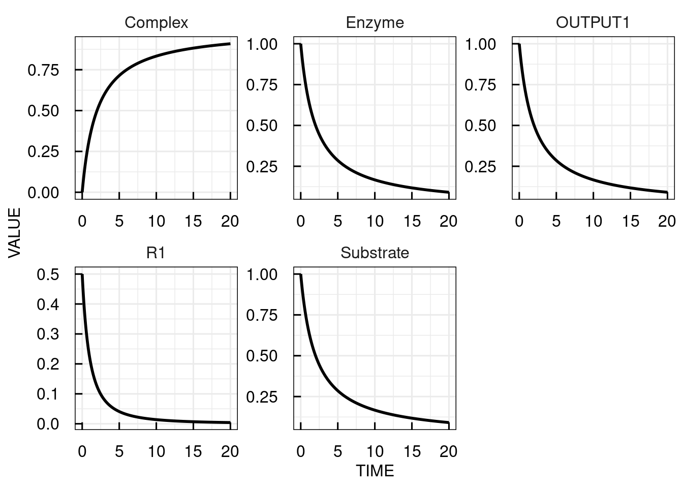

10.2 Simulation settings
The simulation function without further arguments simulates the model with the settings as defined in the model file for a default simulation time of 20 (time units).
To change basic simulation settings, sim_IQRmodel() accepts the following input arguments that are discussed and illustrated in this section.
- simtime
- IC
- parameters
- FLAGoutoutputsOnly
10.2.1 Simulation time
Either a vector with the times at which simuated values should be calculated or a scalar with the maximum simulation time. In the latter case the simulation is evaluated at 1001 time steps between 0 and the maximum simulation time.
10.2.2 Initial conditions
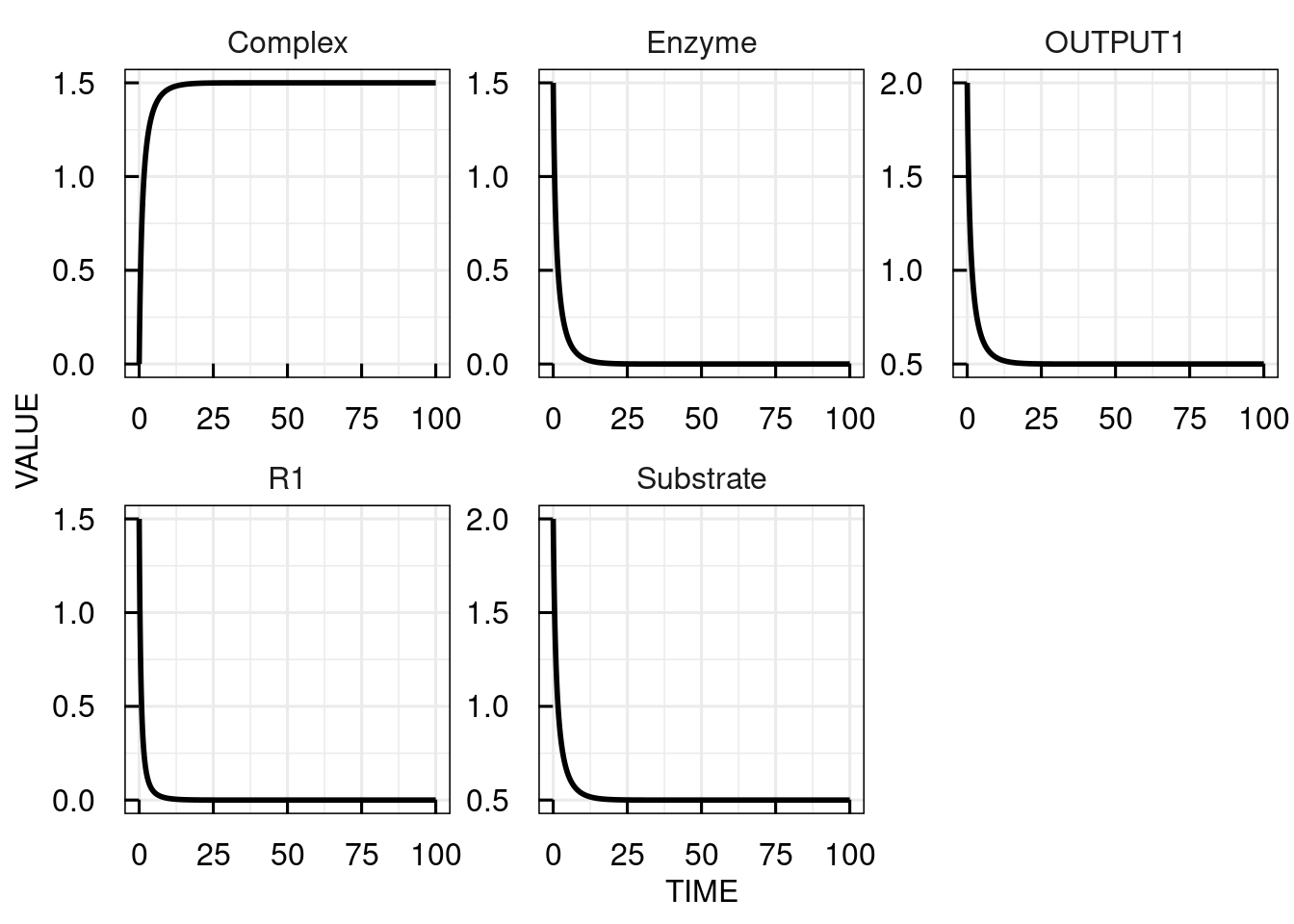
To change the initial conditions of a model we need to specify the initial conditions as a named vector with the names being the state names. When providing initial conditions, values for all states need to be provided.
# Change the ICs for substrate to 2, for the enzyme to 1.5 and simulate the IQRmodel for 100 time units
sim_results2 <- sim_IQRmodel(model,100, IC = c(Substrate= 2, Enzyme = 1.5, Complex = 0))

# plot the simulation results
plot(sim_results2)
10.2.3 Parameters
As for the initial conditions, the parameters need to be given as a named vector. Here, it is possible to set only selected parameters and leave the non-given to the values given in the model. In the following example we simulate the complex formation model with parameter k1 set to 0.2 instead of the default value 0.5.
# Change parameter k1 from 0.5 to 0.2 and simulate the IQRmodel for 100 time units at time steps of 20
sim_results3 <- sim_IQRmodel(model,seq(0,100,20), parameters = c(k1 = 0.2))

# plot the simulation results
plot(sim_results3)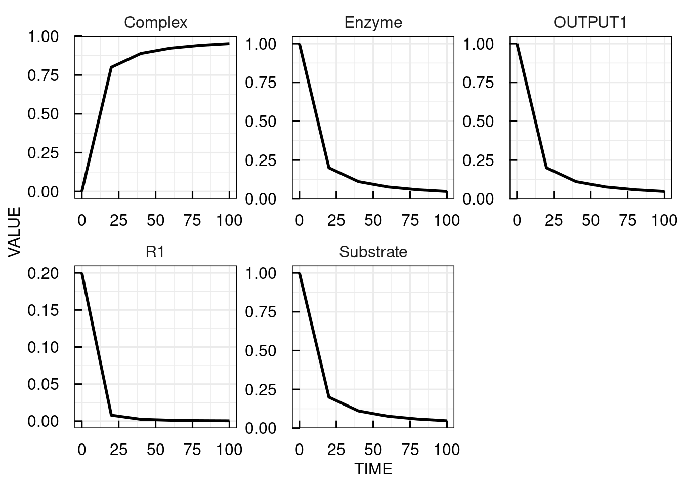

10.2.4 Output selection
Usually, the timecourses of all states, variables, and reactions are returned.
IQRmodels can have outputs explicitely defined (i.e., variables named OUTPUT1, OUTPUT2, OUTPUT3, … in the MODEL VARIABLES section).
Then, we can use the flag FLAGoutputsOnly = TRUE to return these outputs only.
# simulate the IQRmodel for 100 time units and  return the outputs only
sim_results <- sim_IQRmodel(model,100, FLAGoutputsOnly = TRUE)

# plot the simulation results
plot(sim_results)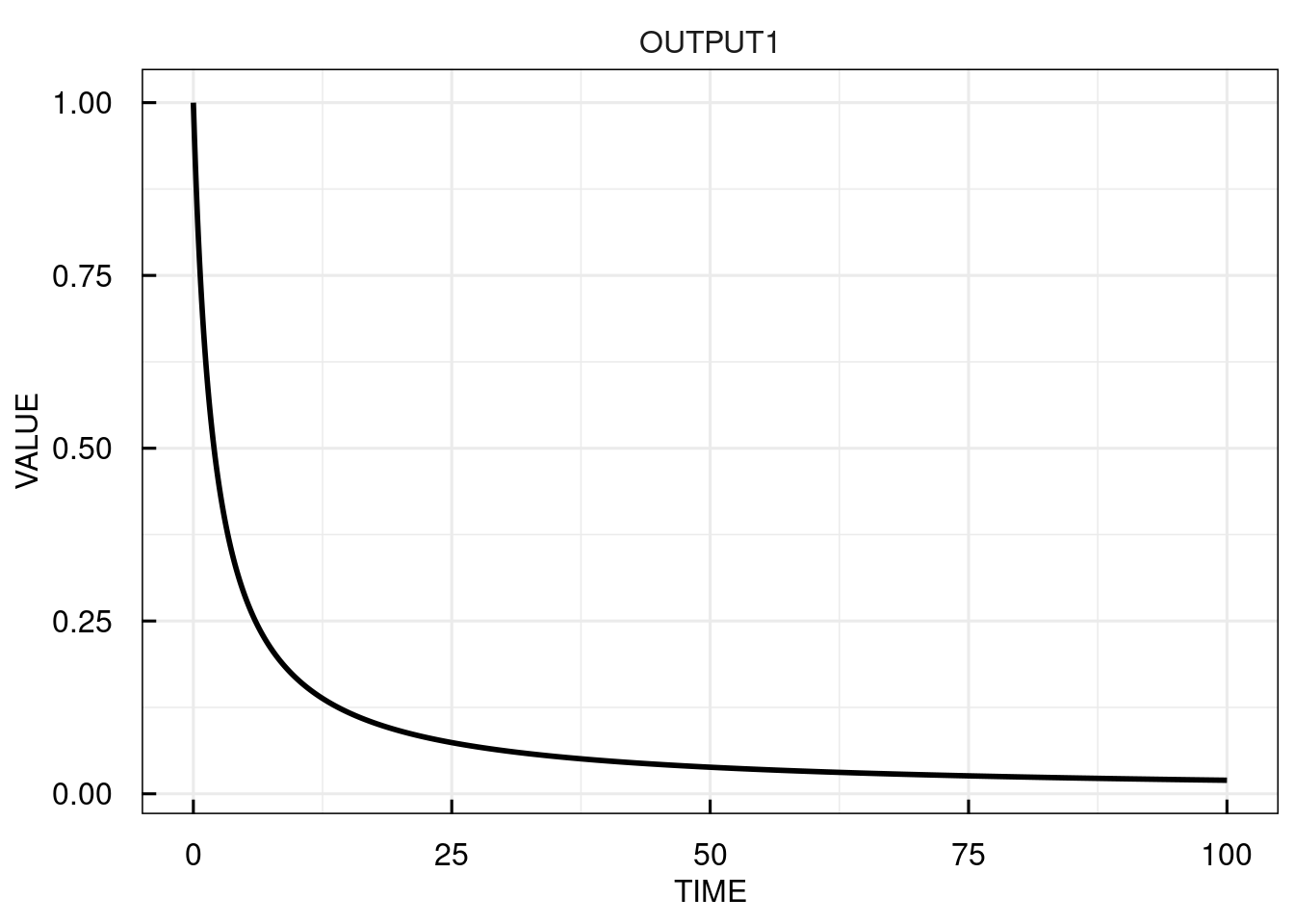

10.3 Dosing events
Pharmacometric and systems pharmacology applications typically include dosing events.
To simulate a model with a dosing event, (i) model inputs needs to be specified in the model and (ii) the dosing event needs to be specified.
Model inputs (i.e., variables INPUT1, INPUT2, INPUT3, …) define the compartment (amount of drug) to which the dose is administered.
Dosing events are defined with the function IQRdosing(), which as a minimum requires the time of dosing (TIME), the dose amount (AMT), and the input number (ADM) to be specified as function arguments.
The additional arguments II and ADDL can be used to define dose-repetitions for a specific dosing event.
II defines the dosing interval and ADDL the number of additional doses.
To implement an infusion instead of a bolus administration, either the infusion time (TINF) or the infusion rate (RATE) can be specified.
For multiple dosing events, the information on time, amount, etc is simply concatenated in vectors (or defined using II and ADDL).
Below, some examples for dosing regimens are shown.
# Define single dose of 10 for INPUT1 at time = 0
dosing <- IQRdosing(TIME = 0, ADM = 1, AMT = 10)

# Define the 4 increasing doses with interval of 12 to INPUT1 and single dose of 20 to INPUT2
dosing <- IQRdosing(TIME = c(0, 12, 24, 36, 0), ADM = c(1, 1, 1, 1, 2), AMT = c(1, 2, 4, 8, 20))


# Define infusion of a dose of 10 over an infusion time of 7
dosing <- IQRdosing(TIME = 0, ADM = 1, AMT = 10, TINF = 7)

# Define o.d. dosing for 1 week
dosing <- IQRdosing(TIME = 0, ADM = 1, AMT = 10, ADDL = 6, II = 24)
Note that the use of model inputs is not restricted to dosing events for pharmacometric model, but can be used in general in cases state variables are instantaneously increased by an external event. For example, the addition of substrates to (bio-)chemical reactions in a test tube could be implemented.
10.3.1 Single dosing input
For simulating models with dosing events, the IQRdosing object is passed to the simulation function as argument dosingTable.
For illustration we use a one-compartmental linear PK model with an model input INPUT1 to the central compartment.
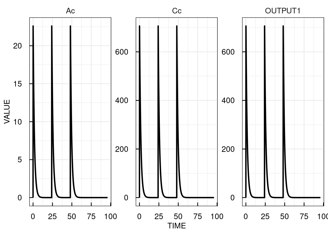
Here, we simulate three doses of 10 with an interval of 24.
# load model
filename <- "material/01-03-BasicSimulation/model_Example2.txt"
model <- IQRmodel(filename)

# Define repeated dose with interval of 24 (hours)
dosing <- IQRdosing(TIME=0,ADM=1,AMT=24,II=24,ADDL=2)

# Simulate model for 96 time units
sim_results <- sim_IQRmodel(model,96,dosingTable=dosing)

# Plot the simulation results for the central compartment
plot(sim_results)
10.3.2 Multiple dosing inputs
To simulate a model with more than one dosing input, the input ADM becomes important to define to which input the respective dose should be added.
This way in the same vectors for the argments TIME, ADM, and AMT to the IQRdosing() function we, e.g., can specify two different administration routes or administration of different compounds.
For example, in a model with two dosing inputs we refer to the dosing input with a dosing input number (1 for INPUT1 and 2 for INPUT2) in ADM, the time points of each event in TIME,
and the amount of the drug per dosing event in AMT.
We extended the one-comartmental PK model with a dosing compartment for oral absorption with 1st order kinetics.
Now, INPUT1 is used for oral dosing. The INPUT2 is added to the central compartment.
In the example below, we implement two oral doses at time 0 and 12 and two infusions with infusion time 3 at times 0 and 15.
# Load model
filename <- "material/01-03-BasicSimulation/model_Example3.txt"
model <- IQRmodel(filename)

# Define the dosing scheme
dosing <- IQRdosing(TIME=c(0,12,0,15),ADM=c(1,1,2,2),AMT=c(5,10,5,15),TINF = c(0,0,3,3))

# Simulate model for 50 time units
sim_results <- sim_IQRmodel(model,50,dosingTable=dosing)

# Plot the simulation results for the central compartment
plot(sim_results)
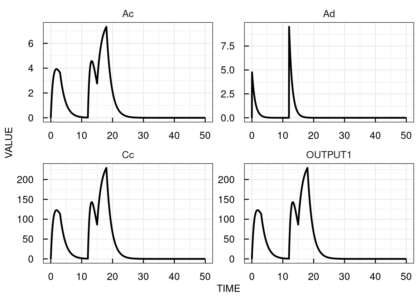
The plots for the bolus dosing inputs (INPUT1) are shown as 0 at all times (since corresponding to instant increases in the state variable values at discrete time points)
while the infusion input (INPUT2) assumes the respective infusion rate for each infusion.
10.3.3 Special dosing parameters
- If
INPUT*definitions are present in a model, the model should contain anINPUT*parameter. “*” in this case represents the numeric number of the input. If such a parameter is not present in the model text description, then it will be added to the model automatically during model import. - For each
INPUT*definition also aTlag*parameter needs to be present in the model. This parameter represent the lagtime for this input. If not present in the model text descriptions, it will be added automatically during the model import and assigned a value of 0 (no lagtime).
10.4 Parameter sensitivities
Confidence in the model predictions in general depends on the confidence in the model parameters.
However, in quantitative terms, a change in a certain parameter may have a large or small effect on a particular model prediction.
Thus, investigating the sensitivities of the model w.r.t. the model parameters is an important aspect for result evaluation and interpretation..
This is especially true for model predictions based on a single optimal parameter point.
In IQR Tools, parameter sensitivity trajectories are computed by setting the flag FLAGsensitivity = TRUE.
# simulate model for 100 time units
sim_results <- sim_IQRmodel(model,50,dosingTable=dosing,FLAGsensitivity=TRUE, sensParams = c("CL"))

# plot the sensitivities over time
plot(attributes(sim_results)$sensitivity)
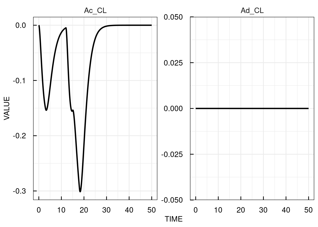
The sensitivities are computed and plotted over time for each of the state variables with respect to the parameter specified in sensParams (CL).
If no parameters are specified, the sensitivity for all are calculated.
The sensitivities from the underlying ODE solver (CVODE) are returned without additional arguments, but it is also possible to use the analytic solutions of the ODE sensitivity equations
(if these can be derived) to compute sensitivities using the flag FLAGuseSensEq = TRUE.
# simulate model for 100 time units
sim_results <- sim_IQRmodel(model,50,dosingTable=dosing,FLAGsensitivity=TRUE, FLAGuseSensEq = TRUE, sensParams = c("CL"))

# plot the sensitivities over time
plot(attributes(sim_results)$sensitivity)

10.5 Integrator in C
The CVODES integrator is used in IQR Tools in order to bring the simulation performance to an adequate level for even the most complex clinical trial simulations. Note that an IQRmodel object already contains the C-compiled version of the model, i.e., the path to the compiled model.