
14 Advanced modeling workflows
14.1 PopPK workflow
This example will go through each step of the model development: from data programming to final modeling report. It demonstrates how to perform a complete population pharmacokinetic (PopPK) analysis using IQR Tools.
14.1.1 Original dataset
In our example, the dataset contains 2 studies:
A single ascending dose study (placebo + 8 active dose groups, 6 subjects (male only) per group)
Multiple ascending dose study (placebo + 4 active dose groups, 10 subjects (male and female) per group)
Some inclusion criteria:
Healthy males between 18 and 40 years of age
Healthy females between 40 and 60 years of age
The simulated dataset is intentionally kept small to allow for acceptable runtimes for demonstration and training purposes. In addition, some outliers and typos have been introduced manually into the dataset (after simulation) in order to demonstrate the data cleaning steps of the workflow.
The dataset is provided as a comma separated file and can be imported directly using the following command:
# Define dataset location
dataFile <- "material/01-06-X1-PopPK/DataSet_Example.csv"
sourceData <- read.csv(dataFile)
The dataset has now been successfully imported.
| USUBJID | STUDY | CENTER | SUBJECT | PART | IND | INDNAME | TRT | TRTNAME | VISIT | VISITNAM | BASE | SCREEN | DATEDAY | DATETIME | NT | TIME | TIMEUNIT | TYPE | TYPENAME | SUBTYPE | VALUE | VALUETXT | UNIT | NAME | DURATION | ULOQ | LLOQ | ROUTE | INTERVAL | NRDOSES |
|---|---|---|---|---|---|---|---|---|---|---|---|---|---|---|---|---|---|---|---|---|---|---|---|---|---|---|---|---|---|---|
| X3401_0100_0001 | 3401 | 100 | 1 | 0 | 0 | Healthy Volunteers | 34010 | Placebo oral single dose | 1 | VISIT 1 - Screening | 0 | 1 | 05-Mar-14 | 09:18 | -168.00 | -168.65 | Hours | 5 | Demographics | 1 | 1.00 | male | . | Gender | 0 | . | . | Oral | . | . |
| X3401_0100_0001 | 3401 | 100 | 1 | 0 | 0 | Healthy Volunteers | 34010 | Placebo oral single dose | 1 | VISIT 1 - Screening | 0 | 1 | 05-Mar-14 | 09:18 | -168.00 | -168.65 | Hours | 5 | Demographics | 2 | 36.00 | 36 | Years | Age | 0 | . | . | Oral | . | . |
| X3401_0100_0001 | 3401 | 100 | 1 | 0 | 0 | Healthy Volunteers | 34010 | Placebo oral single dose | 2 | VISIT 2 - BASELINE / FIRST DOSING DAY | 1 | 0 | 12-Mar-14 | 08:56 | -1.00 | -1.00 | Hours | 6 | Body | 1 | 84.00 | 84 | kg | Bodyweight | 0 | . | . | Oral | . | . |
| X3401_0100_0001 | 3401 | 100 | 1 | 0 | 0 | Healthy Volunteers | 34010 | Placebo oral single dose | 2 | VISIT 2 - BASELINE / FIRST DOSING DAY | 1 | 0 | 12-Mar-14 | 08:56 | -1.00 | -1.00 | Hours | 6 | Body | 2 | 182.00 | 182 | cm | Height | 0 | . | . | Oral | . | . |
| X3401_0100_0001 | 3401 | 100 | 1 | 0 | 0 | Healthy Volunteers | 34010 | Placebo oral single dose | 2 | VISIT 2 - BASELINE / FIRST DOSING DAY | 1 | 0 | 12-Mar-14 | 08:56 | -1.00 | -1.00 | Hours | 6 | Body | 3 | 25.36 | 25.36 | kg/m2 | BMI | 0 | . | . | Oral | . | . |
| X3401_0100_0001 | 3401 | 100 | 1 | 0 | 0 | Healthy Volunteers | 34010 | Placebo oral single dose | 2 | VISIT 2 - BASELINE / FIRST DOSING DAY | 0 | 0 | 12-Mar-14 | 09:52 | -0.08 | -0.08 | Hours | 1 | PK | 1 | 0.00 | 0 | ng/ml | X plasma concentration | 0 | . | 1 | Oral | . | . |
| X3401_0100_0001 | 3401 | 100 | 1 | 0 | 0 | Healthy Volunteers | 34010 | Placebo oral single dose | 2 | VISIT 2 - BASELINE / FIRST DOSING DAY | 0 | 0 | 12-Mar-14 | 09:56 | 0.00 | 0.00 | Hours | 0 | Dose | 1 | 0.00 | 0 | ug | Dose compound X | 0 | . | . | Oral | . | . |
| X3401_0100_0001 | 3401 | 100 | 1 | 0 | 0 | Healthy Volunteers | 34010 | Placebo oral single dose | 2 | VISIT 2 - BASELINE / FIRST DOSING DAY | 0 | 0 | 12-Mar-14 | 10:01 | 0.08 | 0.08 | Hours | 1 | PK | 1 | 0.00 | 0 | ng/ml | X plasma concentration | 0 | . | 1 | Oral | . | . |
| X3401_0100_0001 | 3401 | 100 | 1 | 0 | 0 | Healthy Volunteers | 34010 | Placebo oral single dose | 2 | VISIT 2 - BASELINE / FIRST DOSING DAY | 0 | 0 | 12-Mar-14 | 10:11 | 0.25 | 0.25 | Hours | 1 | PK | 1 | 0.00 | 0 | ng/ml | X plasma concentration | 0 | . | 1 | Oral | . | . |
| X3401_0100_0001 | 3401 | 100 | 1 | 0 | 0 | Healthy Volunteers | 34010 | Placebo oral single dose | 2 | VISIT 2 - BASELINE / FIRST DOSING DAY | 0 | 0 | 12-Mar-14 | 10:26 | 0.50 | 0.50 | Hours | 1 | PK | 1 | 0.00 | 0 | ng/ml | X plasma concentration | 0 | . | 1 | Oral | . | . |
Then, the .csv file needs to be exported in the standardized General Dataset Format (GDF).
In model-based drug development, a GDF minimizes redundancy, reduces errors, and supports multiple pharmacometric analyses across projects and tools. IQR Tools are designed to work directly with this format, ensuring flexibility and consistency.
# Define the names (NAME column) of the records you want to consider as dose records
doseNAMES <- "Dose compound X"

# Define the names (NAME column) of the records you want to consider as observation records
obsNAMES <- "X plasma concentration"

# Define continuous covariates
cov0 <- c(
  WT0 = "Bodyweight",
  AGE0 = "Age",
  HT0 = "Height",
  BMI0 = "BMI"
)

# Define categorical covariates
cat0 <- c(
  SEX = "Gender"
)

# Run IQRdataGENERAL
data1 <- IQRdataGENERAL(
  input = sourceData,
  doseNAMES = "Dose compound X",
  obsNAMES = "X plasma concentration",
  cov0 = cov0,
  cat0 = cat0
)
The resulting data object data1 includes additional columns required for model-based analyses. Some key columns that have been created are:
EVID, indicating dosing events (EVID = 1) and observation records (EVID = 0),
YTYPE, distinguishing between different observation types,
ADM, identifying different dosing types,
AMT, specifying the dosing amount,
MDV, flagging missing observation values (MDV = 1),
CENS, flagging values outside the measurable range (e.g., CENS = 1 for BLQ values),
IXGDF, providing a unique record identifier for each row.
Covariate columns such as WT0, HT0, AGE0,BMI0 and SEXhave also been added, containing numerical values.
The object data1 has been assigned the class IQRdataGENERAL, which stores metadata in its attributes, including information about units, categories, and covariate names. The power of such an approach can easily be seen when using the following functions on an IQRdataGENERAL object - producing report ready demographic summary tables directly from the dataset: summaryCov_IQRdataGENERAL() and summaryCat_IQRdataGENERAL(). More about this in the next section.
14.1.1.1 Data exploration
These two functions are used to create a summary table of demographic data, covering both continuous and categorical covariates.
##    Summary of demographic and baseline characteristics for continuous information
##    ====================================================================================
##
##    Characteristic  | 3401 [N=54]                     | 3402 [N=50]
##    ------------------------------------------------------------------------------------
##    Bodyweight (kg) | 78.7 (7.59) [60-98]             | 71.8 (11.9) [40-91]
##    Age (Years)     | 30 (5.29) [20-44]               | 37.5 (9.43) [21-57]
##    Height (cm)     | 177 (4.54) [169-186] (3 n.a.**) | 171 (9.08) [151-191] (3 n.a.**)
##    BMI (kg/m2)     | 25 (2.11) [19.2-32] (3 n.a.**)  | 24.4 (3.12) [17.5-32] (3 n.a.**)
##    ------------------------------------------------------------------------------------
## N: Number of subjects
## Entries represent: Mean (Standard deviation) [Minimum-Maximum]
## ** missing values in dataset
##
## IQRoutputTable object## Summary of demographic and baseline characteristics for categorical information
## ==================================================================================
##
## Characteristic | Category | 3401 [N=54] | 3402 [N=50]
## ----------------------------------------------------------------------------------
## Gender | male | 50 (92.6%) | 24 (48%)
## | female | 0 (0%) | 25 (50%)
## | n.a.** | 4 (7.41%) | 1 (2%)
## Study | 3401 | 54 (100%) | 0 (0%)
## | 3402 | 0 (0%) | 50 (100%)
## TRTNAME | Placebo oral single dose | 6 (11.1%) | 0 (0%)
## | 1mg oral single dose | 6 (11.1%) | 0 (0%)
## | 2mg oral single dose | 6 (11.1%) | 0 (0%)
## | 5mg oral single dose | 6 (11.1%) | 0 (0%)
## | 10mg oral single dose | 6 (11.1%) | 0 (0%)
## | 20mg oral single dose | 6 (11.1%) | 0 (0%)
## | 50mg oral single dose | 6 (11.1%) | 0 (0%)
## | 100mg oral single dose | 6 (11.1%) | 0 (0%)
## | 200mg oral single dose | 6 (11.1%) | 0 (0%)
## | Placebo oral daily dosing for 28 days | 0 (0%) | 10 (20%)
## | 10mg oral daily dosing for 28 days | 0 (0%) | 10 (20%)
## | 20mg oral daily dosing for 28 days | 0 (0%) | 10 (20%)
## | 50mg oral daily dosing for 28 days | 0 (0%) | 10 (20%)
## | 100mg oral daily dosing for 28 days | 0 (0%) | 10 (20%)
## ----------------------------------------------------------------------------------
## N: Number of subjects
## Number of subjects in each category and percentage within this category
## ** missing values in dataset
##
## IQRoutputTable object## INFO | NAME | VALUE
## -------------------------------------------------------------------------------------------------------------------------
## Dose events | Dose compound X | Ntotal: 1454, Nindiv (min/median/max): 1/1/28)
## Observation events (all) | X plasma concentration | Ntotal: 1837, Nindiv (min/median/max): 1/12/24)
## Observation events (MDV=0) | X plasma concentration | Ntotal: 1346, Nindiv (min/median/max): 1/11/23)
## Doses AMT=0 present | ALL dose events | TRUE (N=286)
## Placebo subjects present (AMT=0 or no doses) | ALL dose events | TRUE (N=16)
## IGNORED (MDV=1) observation records present | ALL observation events | TRUE (N=491)
## Subjects without observations (MDV=0) present | ALL observation events | TRUE (N=16)
## Total BLLOQ information | X plasma concentration | N=491 / 26.7%
## Max % BLLOQ values in a subject | X plasma concentration | 8.33%
## BLLOQ handling method | All observation events | M1
## NLME columns containing NA | All events | HT0, BMI0, SEX
## Issues present in the data | Minor | NONE
## Issues present in the data | Warnings | NONE
## Issues present in the data | Errors | NONE
##
##
## IQRoutputTable objectThe main purpose of these tables is to provide a clear overview of the study design (covariates, number of subjects, etc.) and to help identify potential issues in the dataset that should be addressed before starting the analysis.
A recommended step before any data analysis or modeling activity is to visually explore the data. IQR Tools provides a range of standard plotting functions to support this. Here, we use two of them: plotSpaghetti_IQRdataGENERAL(), which produces concentration-time profiles for each subject per treatment group and is very useful for gaining an overview of observation time courses, and plotIndiv_IQRdataGENERAL(), which generates more detailed plots for each individual and saves them in a PDF file.
## Warning: `aes_string()` was deprecated in ggplot2 3.0.0.
## ℹ Please use tidy evaluation idioms with `aes()`.
## ℹ See also `vignette("ggplot2-in-packages")` for more information.
## ℹ The deprecated feature was likely used in the IQRtools package.
##   Please report the issue at <https://github.com/IntiQuan/IQRtools/issues>.
## This warning is displayed once per session.
## Call `lifecycle::last_lifecycle_warnings()` to see where this warning was generated.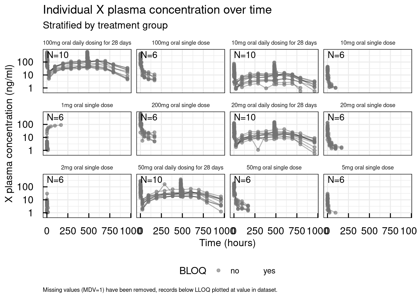
# Generation of a pdf file containing detailed plots for each individual
plotIndiv_IQRdataGENERAL(data1, filename = "material/01-06-X1-PopPK/IndivPlots01.pdf")
From the individual plots, we can identify specific subjects whose observations are implausible or who have outlying records, and these subjects will need to be removed from the analysis. In this case, subjects X3401_0100_0001, X3401_0100_0002, X3401_0100_0003 (and others) are clearly identified as placebo subjects. The plots display the unique subject identifiers, all observations, dosing records, and the treatment group name.
14.1.1.2 Cleaning to create an analysis dataset
removeSubjects <- list("Nonsense profile" = c("X3401_0100_0009"))

removerecords <-  list("Confirmed outlier" = c("268", "860", "1548","2002"))

imputeContinous = c("HT0" = "median", "WT0" = "median", "AGE0" ="median", "BMI0"="median")
imputeCategory =  c("SEX" =1)

dataCleanM1 <- clean_IQRdataGENERAL(data1,
                                    methodBLLOQ = "M1",
                                    subjects = removeSubjects,
                                    records = removerecords,
                                    FLAGrmPlacebo = TRUE,
                                    FLAGrmIGNOREDrecords = FALSE,
                                    continuousCovs = imputeContinous,
                                    categoricalCovs = imputeCategory,
                                    pathname =  "material/01-06-X1-PopPK/DataCLeaning01")

dataCleanM1$STUDYN <- data1$STUDYN[match(dataCleanM1$USUBJID, data1$USUBJID)]
Once the data exploration is complete and the outlier subjects have been identified, we can compile a list of all subjects to be removed from the analysis. Named lists are created, containing either unique subject identifiers (USUBJID) to remove all data from specific subjects or unique record identifiers (IXGDF) to remove particular records. The reasons for removal can vary (e.g., placebo, missing covariates). Additionally, the clean_IQRdataGENERAL() function offers more options and functionality. The arguments continuousCovs and categoricalCovs allow users to impute missing covariate values with values of their choice. In this example, the missing SEX information was set to 1 (male), and all missing continuous covariates were set to the median values within the population in the dataset. Through the vectors imputeContinous and imputeCategory, users can easily specify which covariates to impute and define the corresponding values.
Furthermore, in this example, the method for handling BLOQ (below the limit of quantification) data is set to “M1”, ignored records are retained in the dataset (FLAGrmIGNOREDrecords = FALSE), and placebo subjects are removed (FLAGrmPlacebo = TRUE). Crucially, information on the cleaning process is written to a specified folder, as indicated by the pathname input argument - allowing to include the outputs in this folder directly to the modeling report to document the data transformations.
14.1.1.3 Repeat the general graphical exploration of the cleaned dataset
##    INFO                                        | NAME                   | VALUE
##    -----------------------------------------------------------------------------------------------------------------------
##    Dose events                                 | Dose compound X        | Ntotal: 1167,  Nindiv (min/median/max): 1/1/28)
##    Observation events (all)                    | X plasma concentration | Ntotal: 1513,  Nindiv (min/median/max): 1/12/24)
##    Observation events (MDV=0)                  | X plasma concentration | Ntotal: 1332,  Nindiv (min/median/max): 1/11/23)
##    IGNORED (MDV=1) observation records present | ALL observation events | TRUE (N=181)
##    Total BLLOQ information                     | X plasma concentration | N=177 / 11.7%
##    Max % BLLOQ values in a subject             | X plasma concentration | 8.33%
##    BLLOQ handling method                       | All observation events | M1
##    Issues present in the data                  | Minor                  | NONE
##    Issues present in the data                  | Warnings               | NONE
##    Issues present in the data                  | Errors                 | NONE
##
##
## IQRoutputTable object
# Generation of a pdf file containing detailed plots for each individual
plotIndiv_IQRdataGENERAL(dataCleanM1, filename = "material/01-06-X1-PopPK/IndivPlots02_clean.pdf")Individual profiles and dose-normalized profiles suggest:
- No lag time
- The presence of at least 2 distinct slopes suggests a 2- or 3-compartment model, rather than a 1-compartment model.
14.1.1.4 Export
To prepare the dataset for parameter estimation in NONMEM or MONOLIX, it is exported using the exportNLME_IQRdataGENERAL() function. During this process, certain adjustments are made—such as removing spaces from character strings—to ensure compatibility with the target software.
By default, the function generates a CSV file, but additional export formats can be enabled. Setting FLAGxpt = TRUE will also automatically create an XPT file, while FLAGdefine = TRUE will generate a define file containing specifications for the analysis dataset.
14.1.2 Base Model
To select the appropriate base model, different structural models will be tested and compared. Based on previous assumptions, a 2- or 3-compartment model was suggested; however, a 1-compartment model was also tested here.
The function data_IQRest() is used to define the dataset location, covariates, and dosing information. Meanwhile, modelSpec_IQRest() is used to specify the initial guesses for the typical subject parameters, inter-individual variability (IIV), and error model selection. This function also indicates whether a parameter should be estimated or fixed, specifies the distributions for individual parameters, and applies (time-independent) covariates to parameters.
In the following example, a 1-compartment model was tested. Covariates were defined but not yet implemented in the model. The parameters CL, Vc, and kabs were estimated, along with the IIV, and the error model used was a combined model.
This is an example of how the model should be written, in a .txt file format:
## ********** MODEL NAME
## model_1cpt_linear_abs1
##
## ********** MODEL NOTES
##
## ********** MODEL STATES
##
## d/dt(Ad)    = -kabs*Ad + Fabs1*INPUT1
## d/dt(Ac)    =  kabs*Ad - CL/Vc*Ac
##
## Ad(0)       = 0
## Ac(0)       = 0
##
## ********** MODEL PARAMETERS
##
## Fabs1       = 1   # Relative bioavailability (-)
## kabs        = 2   # Absorption rate parameter (1/hour)
## CL          = 3   # Apparent clearance (L/hour)
## Vc          = 32  # Apparent central volume (L)
## Tlag1       = 0   # Absorption lag time (hours)
##
## ********** MODEL VARIABLES
##
## % Calculation of concentration in central compartment
## Cc          = Ac/Vc
##
## % Defining an output (only needed when interfacing with NLME
## % parameter estimation tools such as NONMEM and MONOLIX)
## OUTPUT1     = Cc  # Compound concentration
##
## ********** MODEL REACTIONS
##
##
## ********** MODEL FUNCTIONS
##
##
## ********** MODEL EVENTS
filename <- "material/01-06-X1-PopPK/basemodel_Example1.txt"
# define dataset location and covariates
data_modeling <- data_IQRest(
datafile = "material/01-06-X1-PopPK/dataNLME01/data.csv" ,
covNames = c("WT0", "AGE0", "BMI0"),
catNames = c("SEX")
)
# Define dosing
dosing <- dosing_IQRest(INPUT1 = c(type ="BOLUS"))
# Model specification: Initial guesses (minimum requirement)
modelSpec <- modelSpec_IQRest(
# Typical subject parameters
POPvalues0 = c(CL = 10, Vc = 100, kabs = 1),
POPestimate= c(CL = 1, Vc = 1, kabs = 1),
# Between subject variability
IIVvalues0=c( CL = 0.5, Vc = 0.5, kabs = 0.5),
IIVestimate=c(CL = 1, Vc = 1, kabs = 1),
# Error model
errorModel=list(OUTPUT1=c(type="absrel", rel0=0.2, abs=0.2))
est1 <- IQRnlmeEst(filename,
dosing,
data_modeling,
modelSpec = modelSpec)
proj_est1 <- IQRnlmeProject(est1,
comment = "1cpt model abs1 & dosing bolus, absrel error, IIV on all",
projectPath = "material/01-06-X1-PopPK/basemodel_Example1",
tool = "NONMEM")
)After definition of the above elements (data, model, dosing, and modelSpec), the IQRnlmeEst() function is used to generate an NLME estimation object.
Definition of the 2-compartment model :
modelSpec <- modelSpec_IQRest(

  # Typical subject parameters
  POPvalues0 = c(CL = 10, Vc = 100, kabs = 1, Q1=10, Vp1=500),
  POPestimate= c(CL = 1,  Vc = 1,   kabs = 1, Q1=1,  Vp1=1),

  # Between subject variability
  IIVvalues0=c(CL = 0.5, Vc = 0.5, kabs = 0.5, Q1=0.5, Vp1=0.5),
  IIVestimate=c(CL = 1,  Vc = 1,   kabs = 1,   Q1=1,   Vp1=1),

  # Error model
  errorModel=list(OUTPUT1=c(type="absrel",  rel0=0.2, abs=0.2))
)
proj_est2 <- IQRnlmeProject(est2,
comment = "2cpt model abs1 & dosing bolus, absrel error, IIV on all",
projectPath = "material/01-06-X1-PopPK/basemodel_Example2",
tool = "NONMEM")Definition of the 3-compartment model :
# Model specification: Initial guesses (minimum requirement)
modelSpec <- modelSpec_IQRest(

# Typical subject parameters

  POPvalues0 = c(CL = 10, Vc = 100, kabs = 1, Q1=10, Vp1=500, Q2=10, Vp2=500),
  POPestimate= c(CL = 1,  Vc = 1,   kabs = 1, Q1=1,  Vp1=1,   Q2=1,  Vp2=1),

  # Between subject variability
  IIVvalues0=c( CL = 0.5, Vc = 0.5, kabs = 0.5, Q1=0.5, Vp1=0.5, Q2=0.5, Vp2=0.5),
  IIVestimate=c(CL = 1,   Vc = 1,   kabs = 1,   Q1=1,   Vp1=1,   Q2=1,   Vp2=1),

  # Error model
  errorModel=list(OUTPUT1=c(type="absrel",  rel0=0.2, abs=0.2))
)
proj_est3 <- IQRnlmeProject(est3,
comment = "3cpt model abs1 & dosing bolus, absrel error, IIV on all",
projectPath = "material/01-06-X1-PopPK/basemodel_Example3",
tool = "NONMEM")The same approach was applied to the 2-compartment and 3-compartment models. The only difference between the projects was in the model definition step, where additional parameters needed to be added due to the change in the number of compartments-and the project path, which had to be updated based on specific example.
## <TT>   Comparison of model results for multiple models
##        ==========================================================================
##
## <TH>   Parameter   | basemodel_Example1 | basemodel_Example2 | basemodel_Example3
##        --------------------------------------------------------------------------
## <TR>   kabs        | 3.26 (7.2%)        | 2.08 (4%)          | 1.96 (7%)
## <TR>   CL          | 30.8 (7.1%)        | 23.3 (4.7%)        | 22.9 (5%)
## <TR>   Vc          | 283 (5.1%)         | 210 (4.1%)         | 199 (6.2%)
## <TR>   Q1          | -                  | 22.6 (3.7%)        | 4.67 (47%)
## <TR>   Vp1         | -                  | 2110 (4.5%)        | 709 (4.2%)
## <TR>   Q2          | -                  | -                  | 17.3 (12%)
## <TR>   Vp2         | -                  | -                  | 1590 (8.6%)
## <TR>               |                    |                    |
## <TR>   omega(kabs) | 0.233 (34%)        | 0.316 (8.7%)       | 0.434 (10%)
## <TR>   omega(CL)   | 0.381 (15%)        | 0.345 (11%)        | 0.347 (12%)
## <TR>   omega(Vc)   | 0.307 (8.6%)       | 0.334 (7%)         | 0.414 (9.9%)
## <TR>   omega(Q1)   | -                  | 0.276 (9.2%)       | 0.83 (31%)
## <TR>   omega(Vp1)  | -                  | 0.271 (12%)        | 0.0198 (180%)
## <TR>   omega(Q2)   | -                  | -                  | 0.246 (21%)
## <TR>   omega(Vp2)  | -                  | -                  | 0.356 (20%)
## <TR>               |                    |                    |
## <TR>   error_ADD1  | 10.4 (1.1%)        | 0.398 (10%)        | 0.394 (10%)
## <TR>   error_PROP1 | 0.246 (2.8%)       | 0.109 (2.8%)       | 0.11 (2.8%)
## <TR>               |                    |                    |
## <TR>   OBJ         | 9275               | 5699               | 5759
## <TR>   BIC         | 9333               | 5785               | 5874
## <TR>   AIC         | 9291               | 5723               | 5791
##        --------------------------------------------------------------------------
## <TF>    FIX (parameter fixed to this value), - (parameter not used)<br>Number of significant digits: 3.<br>Relative standard errors (RSE) given in parenthesis with 2 significant digits.<br>Model metrics (OBJ, AIC, BIC) are rounded to nearest integer., basemodel_Example1 (material/01-06-X1-PopPK/basemodel_Example1), basemodel_Example2 (material/01-06-X1-PopPK/basemodel_Example2), basemodel_Example3 (material/01-06-X1-PopPK/basemodel_Example3)
Subsequently, the three NLME projects (1-compartment, 2-compartment, and 3-compartment models) were created and run, allowing for comparison between them to select the best model based on the objective function value (OBJ), AIC, and BIC.
It is assumed that all individual PK model parameters are log-normally distributed throughout this example. The two compartmental distribution model was considered further.
14.1.3 Error model
To implement an error model in the base model, the script follows a similar structure. The user can choose between an additive (abs), proportional (rel) or combined (absrel) error model. In this case, basemodel_Example2 was chosen for the subsequent steps of the analysis.
## <TT>   Comparison of model results for multiple models
##        =======================================================
##
## <TH>   Parameter   | errormodel_Example1 | errormodel_Example2
##        -------------------------------------------------------
## <TR>   kabs        | 2.1 (4.1%)          | 2.08 (4%)
## <TR>   CL          | 22.7 (4.7%)         | 23.3 (4.7%)
## <TR>   Vc          | 211 (4.1%)          | 210 (4.1%)
## <TR>   Q1          | 22.7 (3.9%)         | 22.6 (3.7%)
## <TR>   Vp1         | 2110 (4.5%)         | 2110 (4.5%)
## <TR>               |                     |
## <TR>   omega(kabs) | 0.314 (9.1%)        | 0.316 (8.7%)
## <TR>   omega(CL)   | 0.362 (11%)         | 0.345 (11%)
## <TR>   omega(Vc)   | 0.336 (7%)          | 0.334 (7%)
## <TR>   omega(Q1)   | 0.3 (9.2%)          | 0.276 (9.2%)
## <TR>   omega(Vp1)  | 0.279 (12%)         | 0.271 (12%)
## <TR>               |                     |
## <TR>   error_PROP1 | 0.125 (2%)          | 0.109 (2.8%)
## <TR>   error_ADD1  | -                   | 0.398 (10%)
## <TR>               |                     |
## <TR>   OBJ         | 5799                | 5699
## <TR>   BIC         | 5878                | 5785
## <TR>   AIC         | 5821                | 5723
##        -------------------------------------------------------
## <TF>    FIX (parameter fixed to this value), - (parameter not used)<br>Number of significant digits: 3.<br>Relative standard errors (RSE) given in parenthesis with 2 significant digits.<br>Model metrics (OBJ, AIC, BIC) are rounded to nearest integer., errormodel_Example1 (material/01-06-X1-PopPK/errormodel_Example1), errormodel_Example2 (material/01-06-X1-PopPK/errormodel_Example2)
According to the results, both the OBJ and BIC values were lower when using the combined error model (additive + proportional). Since this model is nested within simpler error models, the BIC—being more conservative and penalizing complexity—is the preferred criterion for comparison.
Decision about the base model:
- No lag time
- Linear elimination
- 2 compartments
- Additive+proportional error model
- Random effects on all the PK parameters in this model seem identifiable
14.1.4 Covariate model building
The covariates will be assessed in several steps, using the full covariate modeling (FCM) approach, rather than stepwise covariate modeling (though the exact mechanism of this FCM is not reported here, but will be discussed in a later chapter).
Step 1: Discussions on which candidate covariates are of clinical interest. Selecting these and specifying them in the modeling plan
Which candidate covariates and on which parameters each of these covariates should be tested.
Here in this case, AGE0 and SEX are of interest to test on CL, due to what is known about the metabolism of the compound.
It is assumed that the clinical team is more interested in using WT0 as covariate than HT0 or BMI0. Thus WT0 will be tested on all PK parameters, except ka.
Correlations of ETAs with covariates also suggest to test AGE0 and SEX on Vc.
Step 2: Consider the correlations between the retained candidate covariates. - No need to test BMI0 and HT0 and WT0, but only one of them.
Step 3: Perform a single estimation run where all candidate covariates of interest are tested on all parameters. The selection of candidate covariates might be parameter dependent as discussed above. - Separate covariate coefficients will be estimated for each covariate relationship
Step 4: Analyze the results
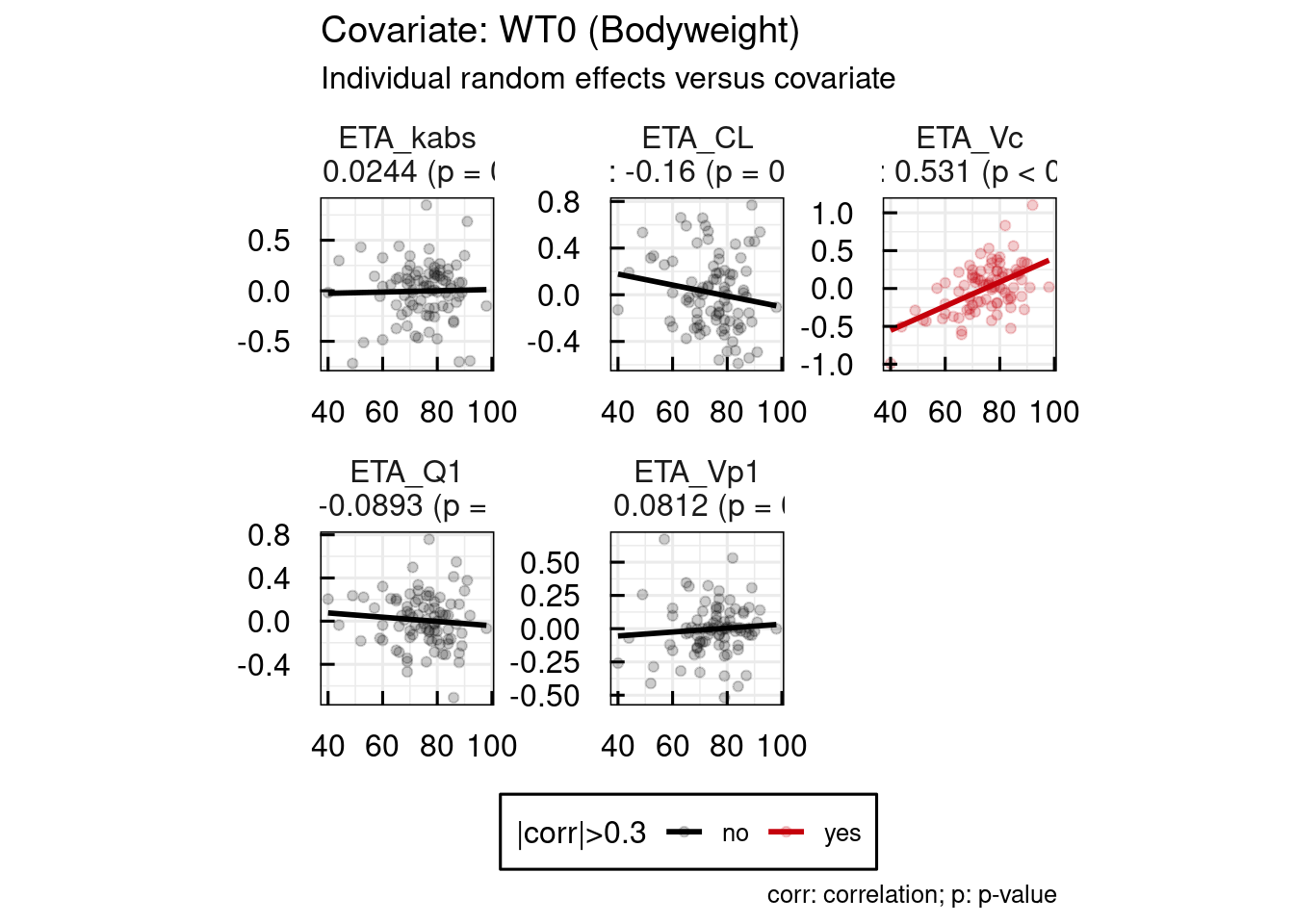
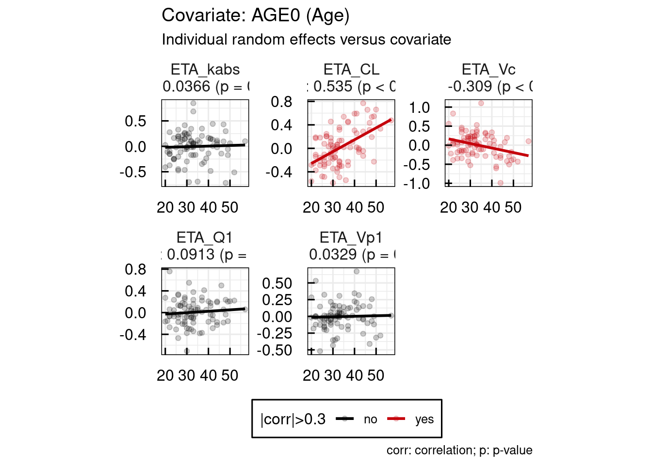
When a covariate is implemented in a model, various diagnostic plots can be used to assess its relevance. One key tool is the ETA vs COV plots, which display the relationship between the individual random effects (ETAs) of a parameter and a specific covariate. A visible correlation in these plots (assuming a small to moderate shrinkage) may suggest that the covariate explains part of the interindividual variability. Conversely, the absence of correlation can indicate that the variability has been adequately captured by the model (again under the assumption of a reasonable shrinkage). The objective is to explore and incorporate covariates that collectively account for most of the variability, ultimately improving model predictability and reducing unexplained interindividual differences.
Examples for ETA vs COV plots are shown below. These plots are also immediately available as PDF documents one an IQRnlmeProject has been run.
# Generate ETA vs Cov plots
project <- as_IQRnlmeProject("material/01-06-X1-PopPK/basemodel_Example2/")
p <-  plot(project)
## Generation of general GoF plots of project: material/01-06-X1-PopPK/basemodel_Example2/
## No covariates present in the model.
## Generation of output specific GoF plots of project: material/01-06-X1-PopPK/basemodel_Example2/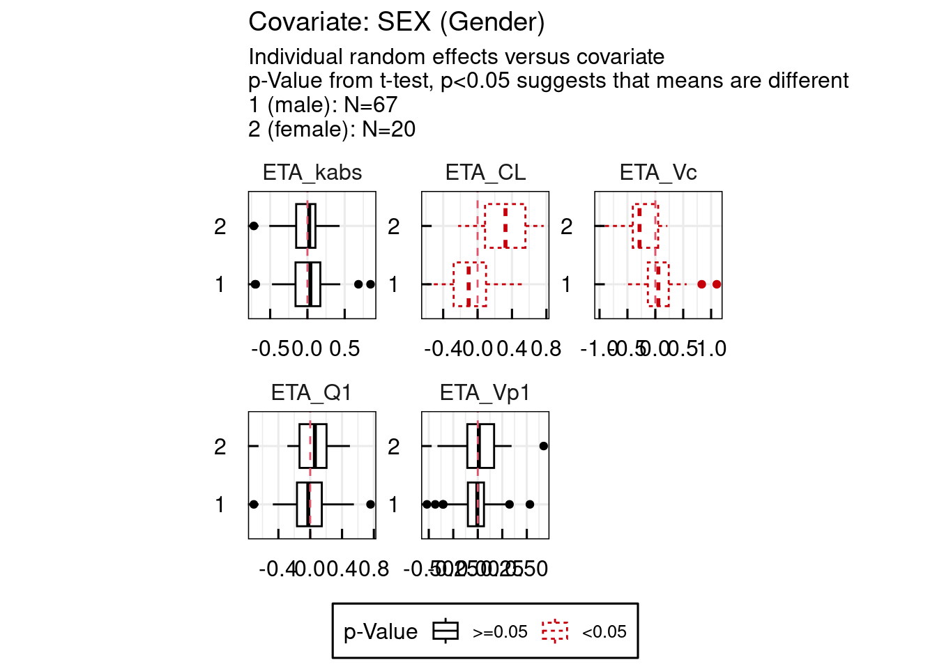
 Example 1 : SEX / HT0 / AGE0 implemented on all parameters except kabs
filename <- "material/01-06-X1-PopPK/basemodel_Example2.txt"

# define dataset location and covariates
data_modeling <- data_IQRest(
  datafile = "material/01-06-X1-PopPK/dataNLME01/data.csv" ,
  covNames  = c("WT0", "AGE0"),
  catNames  = c("SEX")
)

# Define dosing
dosing      <- dosing_IQRest(INPUT1 = c(type ="BOLUS"))

# Model specification: Initial guesses (minimum requirement)
modelSpec <- modelSpec_IQRest(

  # Typical subject parameters
  POPvalues0 = c(CL = 23, Vc = 209, kabs = 1, Q1=23, Vp1=2100),
  POPestimate= c(CL = 1,  Vc = 1,   kabs = 1, Q1=1,  Vp1=1),

  # Between subject variability
  IIVdistribution = c(CL = "L", Vc = "L", kabs = "L", Q1 = "L", Vp1 = "L" ),
  IIVvalues0=c(        CL = 0.5, Vc = 0.5, kabs = 0.5, Q1 = 0.5, Vp1 = 0.5),
  IIVestimate=c(       CL = 1,   Vc = 1,   kabs = 1,   Q1 = 1,   Vp1 = 1),

  # Centering of covariates
  covariateModel = list(CL = c("SEX", "AGE0", "WT0"),
                        Vc = c("SEX", "AGE0", "WT0"),
                        Q1 = c("SEX", "AGE0", "WT0"),
                        Vp1= c("SEX", "AGE0", "WT0")),

  COVcentering = c(SEX=1),

  covariateModelValues = list(CL = c("SEX"=0.4, "AGE0"=0.5, "WT0"=0.75),
                              Vc = c("SEX"=0.4, "AGE0"=0.5, "WT0"=0.75),
                              Q1 = c("SEX"=0.4, "AGE0"=0.5, "WT0"=0.75),
                              Vp1 = c("SEX"=0.4, "AGE0"=0.5, "WT0"=0.75)),

  # Error model
  errorModel=list(OUTPUT1=c(type="absrel",  rel0=0.2, abs=0.2))
)

est2 <- IQRnlmeEst(filename,
                     dosing,
                     data_modeling,
                     modelSpec = modelSpec)


proj_est2   <- IQRnlmeProject(est2,
                          comment = "2cpt model abs1 & dosing bolus, absrel error, IIV on all",
                          projectPath = "material/01-06-X1-PopPK/covariatemodel_Example1",
                          tool = "NONMEM")
Example 2 : SEX implemented on all parameters except kabs
# Centering of covariates
  covariateModel = list(CL = c("SEX"), Vc = c("SEX"), Q1 = c("SEX"), Vp1= c("SEX"))
  COVcentering = c(SEX=1)
  covariateModelValues = list(CL = c("SEX"=0.4),
                              Vc = c("SEX"=0.4),
                              Q1 = c("SEX"=0.4),
                              Vp1 = c("SEX"=0.4))
The presented example illustrates how covariates can be implemented in different ways and compared to select the best covariate model. The selection of covariates will depend on the user, based on the specific case study and the interpretation of the results. Further details on covariate selection will be provided in the dedicated Covariate selection.
## <TT>   Comparison of model results for multiple models
##        ===================================================================
##
## <TH>   Parameter       | covariatemodel_Example1 | covariatemodel_Example2
##        -------------------------------------------------------------------
## <TR>   kabs            | 2.09 (4.6%)             | 2.09 (4.3%)
## <TR>   CL              | 20.6 (5.1%)             | 20.3 (4.9%)
## <TR>   Vc              | 227 (4.9%)              | 229 (5.1%)
## <TR>   Q1              | 22 (4.9%)               | 22.4 (4.1%)
## <TR>   Vp1             | 2070 (8.3%)             | 2090 (5.7%)
## <TR>                   |                         |
## <TR>   omega(kabs)     | 0.321 (8.8%)            | 0.318 (8.6%)
## <TR>   omega(CL)       | 0.275 (13%)             | 0.287 (12%)
## <TR>   omega(Vc)       | 0.281 (11%)             | 0.306 (8.2%)
## <TR>   omega(Q1)       | 0.279 (9.8%)            | 0.282 (9.2%)
## <TR>   omega(Vp1)      | 0.266 (16%)             | 0.269 (14%)
## <TR>                   |                         |
## <TR>   beta_CL(SEX_2)  | 0.539 (26%)             | 0.51 (15%)
## <TR>   beta_CL(AGE0)   | 0.125 (180%)            | -
## <TR>   beta_CL(WT0)    | 0.433 (78%)             | -
## <TR>   beta_Vc(SEX_2)  | -0.209 (76%)            | -0.372 (28%)
## <TR>   beta_Vc(AGE0)   | -0.0394 (520%)          | -
## <TR>   beta_Vc(WT0)    | 0.716 (64%)             | -
## <TR>   beta_Q1(SEX_2)  | 0.151 (140%)            | 0.0606 (190%)
## <TR>   beta_Q1(AGE0)   | -0.174 (130%)           | -
## <TR>   beta_Q1(WT0)    | 0.0681 (580%)           | -
## <TR>   beta_Vp1(SEX_2) | 0.233 (100%)            | 0.0476 (180%)
## <TR>   beta_Vp1(AGE0)  | 0.0252 (1300%)          | -
## <TR>   beta_Vp1(WT0)   | 0.755 (62%)             | -
## <TR>                   |                         |
## <TR>   error_ADD1      | 0.381 (11%)             | 0.386 (11%)
## <TR>   error_PROP1     | 0.109 (3%)              | 0.109 (2.8%)
## <TR>                   |                         |
## <TR>   OBJ             | 5637                    | 5659
## <TR>   BIC             | 5810                    | 5774
## <TR>   AIC             | 5685                    | 5691
##        -------------------------------------------------------------------
## <TF>    FIX (parameter fixed to this value), - (parameter not used)<br>Number of significant digits: 3.<br>Relative standard errors (RSE) given in parenthesis with 2 significant digits.<br>Model metrics (OBJ, AIC, BIC) are rounded to nearest integer., covariatemodel_Example1 (material/01-06-X1-PopPK/covariatemodel_Example1), covariatemodel_Example2 (material/01-06-X1-PopPK/covariatemodel_Example2)
14.1.4.1 Refinement of covariate model
Based on the previous results, the covariate model can be refined. As explained, plots and tables generated during the NLME project guide the user in selecting relevant covariates. In this case, models with different covariate implementations can be compared using the Objective Function Value (OFV), or the Bayesian Information Criterion (BIC - when comparing nested models). In addition, forest plots are another valuable tool for evaluating the impact of covariates on model parameters and assessing their clinical significance. Both the ETA vs covariate plots and forest plots discussed in this section are automatically generated when running an NLME project.
filename <- "material/01-06-X1-PopPK/basemodel_Example2.txt"

# define dataset location and covariates
data_modeling <- data_IQRest(
  datafile = "material/01-06-X1-PopPK/dataNLME01/data.csv" ,
  covNames  = c("WT0", "AGE0"),
  catNames  = c("SEX")
)

# Define dosing
dosing      <- dosing_IQRest(INPUT1 = c(type ="BOLUS"))

# Model specification: Initial guesses (minimum requirement)

modelSpec <- modelSpec_IQRest(

  # Typical subject parameters
  POPvalues0 = c(CL = 23, Vc = 209, kabs = 1, Q1=23, Vp1=2100),
  POPestimate= c(CL = 1,  Vc = 1,  kabs = 1, Q1=1, Vp1=1),

  # Between subject variability
  IIVdistribution = c(CL = "L", Vc = "L", kabs = "L", Q1 = "L", Vp1 = "L" ),
  IIVvalues0=c(       CL = 0.5, Vc = 0.5, kabs = 0.5, Q1 = 0.5, Vp1 = 0.5),
  IIVestimate=c(      CL = 1,   Vc = 1,   kabs = 1,   Q1 = 1,   Vp1 = 1),

  # Centering of covariates
  covariateModel = list(CL = c("SEX", "AGE0", "WT0"),
                        Vc = c("WT0")),
  COVcentering = c(SEX=1),
  covariateModelValues = list(CL = c("SEX"=0.4, "AGE0"=0.5, "WT0"=0.75),
                              Vc = c("WT0"=0.75)),

  # Error model
  errorModel=list(OUTPUT1=c(type="absrel",  rel0=0.2, abs=0.2))
)

est2 <- IQRnlmeEst(filename,
                     dosing,
                     data_modeling,
                     modelSpec = modelSpec)


proj_est2   <- IQRnlmeProject(est2,
                          comment = "2cpt model abs1 & dosing bolus, absrel error, IIV on all",
                          projectPath = "material/01-06-X1-PopPK/covariatemodel_Example3",
                          tool = "NONMEM")
run_IQRnlmeProject(proj_est2)
Examples for covariate impact plots (forest plots), that are automatically generated upon execution of an IQRnlmeProject are shown below.
14.1.5 Covariance model
In this section, several examples will be presented, each illustrating a different approach to constructing the OMEGA covariance matrix. The only required modifications are outlined below and can be directly added to the modelSpec_IQRest() section, as previously discussed.
Example 1:
  # Covariance model
  covarianceModel = c("CL,Vc"),

  # Error model
  errorModel=list(OUTPUT1=c(type="absrel",  rel0=0.2, abs=0.2))
Example 2:
  # covariance model
  covarianceModel = c("CL,Vc","Q1,Vp1"),

  # Error model
  errorModel=list(OUTPUT1=c(type="absrel",  rel0=0.2, abs=0.2))
Example 3:
  # Covariance model
  covarianceModel = c("CL,Vc,kabs,Q1,Vp1")

  # Error model
  errorModel=list(OUTPUT1=c(type="absrel",  rel0=0.2, abs=0.2))
## <TT> Comparison of model results for multiple models
## ===============================================================================================
##
## <TH> Parameter | covariancemodel_Example1 | covariancemodel_Example2 | covariancemodel_Example3
## -----------------------------------------------------------------------------------------------
## <TR> CL | 20.8 (4%) | 20.8 (4%) | 20.2 (4.2%)
## <TR> Vc | 222 (3.6%) | 223 (3.7%) | 220 (4%)
## <TR> kabs | 2.09 (4.2%) | 2.09 (4.2%) | 2.09 (4.8%)
## <TR> Q1 | 22.9 (3.6%) | 22.9 (3.9%) | 22.9 (3.6%)
## <TR> Vp1 | 2130 (4.3%) | 2120 (4.2%) | 2140 (4.4%)
## <TR> | | |
## <TR> omega(CL) | 0.269 (11%) | 0.265 (11%) | 0.27 (12%)
## <TR> omega(Vc) | 0.277 (9.1%) | 0.28 (9.8%) | 0.28 (12%)
## <TR> omega(kabs) | 0.316 (9%) | 0.317 (9%) | 0.314 (9.3%)
## <TR> omega(Q1) | 0.275 (8.8%) | 0.285 (9.7%) | 0.276 (10%)
## <TR> omega(Vp1) | 0.272 (14%) | 0.27 (14%) | 0.269 (14%)
## <TR> | | |
## <TR> beta_CL(SEX_2) | 0.486 (21%) | 0.515 (18%) | 0.62 (19%)
## <TR> beta_CL(AGE0) | 0.407 (46%) | 0.23 (82%) | 0.203 (120%)
## <TR> beta_CL(WT0) | 0.734 (43%) | 0.722 (43%) | 0.702 (47%)
## <TR> beta_Vc(WT0) | 1.25 (20%) | 1.44 (18%) | 1.05 (25%)
## <TR> | | |
## <TR> corr(CL,Vc) | 0.531 (21%) | 0.534 (21%) | 0.467 (28%)
## <TR> corr(Q1,Vp1) | - | 0.16 (130%) | 0.132 (180%)
## <TR> corr(CL,kabs) | - | - | -0.0697 (290%)
## <TR> corr(Vc,kabs) | - | - | -0.0558 (340%)
## <TR> corr(CL,Q1) | - | - | 0.209 (79%)
## <TR> corr(Vc,Q1) | - | - | 0.285 (79%)
## <TR> corr(kabs,Q1) | - | - | 0.112 (160%)
## <TR> corr(CL,Vp1) | - | - | 0.0917 (200%)
## <TR> corr(Vc,Vp1) | - | - | 0.522 (23%)
## <TR> corr(kabs,Vp1) | - | - | -0.0579 (340%)
## <TR> | | |
## <TR> error_ADD1 | 0.391 (10%) | 0.392 (10%) | 0.396 (11%)
## <TR> error_PROP1 | 0.109 (2.8%) | 0.109 (2.8%) | 0.109 (3.2%)
## <TR> | | |
## <TR> OBJ | 5613 | 5613 | 5594
## <TR> BIC | 5735 | 5743 | 5781
## <TR> AIC | 5647 | 5649 | 5646
## -----------------------------------------------------------------------------------------------
## <TF> FIX (parameter fixed to this value), - (parameter not used)<br>Number of significant digits: 3.<br>Relative standard errors (RSE) given in parenthesis with 2 significant digits.<br>Model metrics (OBJ, AIC, BIC) are rounded to nearest integer., covariancemodel_Example1 (material/01-06-X1-PopPK/covariancemodel_Example1), covariancemodel_Example2 (material/01-06-X1-PopPK/covariancemodel_Example2), covariancemodel_Example3 (material/01-06-X1-PopPK/covariancemodel_Example3)Upon comparison, all pairwise ETA correlations involving kabs exhibit very high relative standard errors (RSEs), suggesting poor identifiability. In contrast, acceptable correlations were only observed between CL/Vc and Vc/Vp1. Therefore, Example 4 will use a covariance matrix that includes only these two correlations, as they represent meaningful covariance structures with a noticeable impact.
Example 4:
# covariance model

    covarianceModel = c("CL,Vc,Vp1")
# error model

  errorModel=list(OUTPUT1=c(type="absrel",  rel0=0.2, abs=0.2))
## <TT> Population parameter estimates
## ==========================================================================================================================
##
## <TH> PARAMETER | VALUE | RSE | SHRINKAGE | COMMENT
## --------------------------------------------------------------------------------------------------------------------------
## <TR> **Typical parameters** | | | |
## <TR> CL | 20.7 | 3.92% | - | Apparent clearance (L/hour)
## <TR> Vc | 222 | 3.51% | - | Apparent central volume (L)
## <TR> Q1 | 22.9 | 3.69% | - | Apparent intercompartmental clearance (L/hour)
## <TR> Vp1 | 2120 | 4.43% | - | Apparent peripheral volume (L)
## <TR> kabs | 2.09 | 4.38% | - | Absorption rate parameter (1/hour)
## <TR> | | | |
## <TR> **Inter-individual variability** | | | |
## <TR> omega(CL) | 0.266 | 11.9% | 7.5% | LogNormal
## <TR> omega(Vc) | 0.281 | 9.27% | 3.9% | LogNormal
## <TR> omega(Q1) | 0.277 | 10.3% | 11.4% | LogNormal
## <TR> omega(Vp1) | 0.269 | 13.1% | 21.1% | LogNormal
## <TR> omega(kabs) | 0.314 | 8.98% | 9.6% | LogNormal
## <TR> | | | |
## <TR> **Correlation of random effects** | | | |
## <TR> corr(CL,Vc) | 0.463 | 27.6% | - | Correlation coefficient
## <TR> corr(CL,Q1) | 0.197 | 76.9% | - | Correlation coefficient
## <TR> corr(Vc,Q1) | 0.291 | 70.8% | - | Correlation coefficient
## <TR> corr(CL,Vp1) | 0.102 | 171% | - | Correlation coefficient
## <TR> corr(Vc,Vp1) | 0.555 | 19.2% | - | Correlation coefficient
## <TR> corr(Q1,Vp1) | 0.134 | 159% | - | Correlation coefficient
## <TR> | | | |
## <TR> **Parameter-Covariate relationships** | | | |
## <TR> beta_CL(SEX_2) | 0.537 | 17.7% | - | Gender female on CL
## <TR> beta_CL(AGE0) | 0.309 | 64.8% | - | Age in Years on CL (centered around: 32 Years)
## <TR> beta_CL(WT0) | 0.738 | 41.5% | - | Bodyweight in kg on CL (centered around: 77 kg)
## <TR> beta_Vc(WT0) | 1.27 | 21.7% | - | Bodyweight in kg on Vc (centered around: 77 kg)
## <TR> | | | |
## <TR> **Residual Variability** | | | |
## <TR> error_ADD1 | 0.403 | 10.4% | 12.3%* | Additive Error (ng/ml) - Compound concentration
## <TR> error_PROP1 | 0.109 | 2.99% | - | Proportional Error (fraction) - Compound concentration
## <TR> | | | |
## <TR> Objective function | 5594 | - | - | -
## <TR> AIC | 5638 | - | - | -
## <TR> BIC | 5752 | - | - | -
## --------------------------------------------------------------------------------------------------------------------------
## <TF> Model: material/01-06-X1-PopPK/covariancemodel_Example4, Significant digits: 3 (Objective function rounded to closest integer value), omega values and error model parameters reported in standard deviation.<br>As suggested in the NONMEM manual, the objective function was determined using importance sampling (IMP) with settings EONLY=1 and MAPITER=0.<br>\* Epsilon shrinkage (records with missing dependent variable and censored records not considered).Here the model with the covariance matrix with CL/Vc and Vc/Vp1 is selected. In a popPK modeling task with real data the decision might have been different.
The final popPK model has the following properties:
Linear 2-compartmental distribution model
Linear elimination from central compartment
First order absorption without lag time
Additive+proportional residual error model
Covariance matrix including
CL,VcandVp1SEX,AGE0,WT0as covariates onCLandWT0onVc
14.1.6 Generation of VPCs for final model
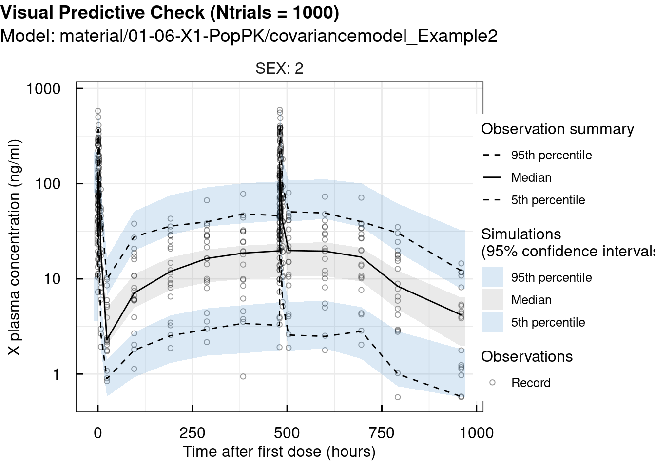
At this point, Visual Predictive Checks (VPCs) were performed using the vpc_IQRnlmeProject() function, which allows easy stratification by SEX and STUDY in this example. VPCs are used to validate the previous steps by comparing the model’s simulations to the observed data.
# standard VPC
vpc_sim <- vpc_IQRnlmeProject(project = "material/01-06-X1-PopPK/covariancemodel_Example2" ,
                              Ntrials = 1000)

vpc_plot <- plotVPC_IQRdataVPC(vpc_sim,
                               stratifyBy = "SEX",
                               FLAGlogY = T,
                               FLAGrmBLQ = T)

print(vpc_plot)
## $OUTPUT1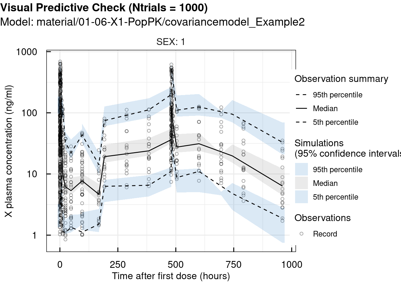
## 2 pages were printed to the graphics device.# standard VPC
vpc_sim <- vpc_IQRnlmeProject(project = "material/01-06-X1-PopPK/covariancemodel_Example2" ,
Ntrials = 1000)
vpc_plot <- plotVPC_IQRdataVPC(vpc_sim,
stratifyBy = "STUDY",
FLAGlogY = T,
FLAGrmBLQ = T)
print(vpc_plot)## $OUTPUT1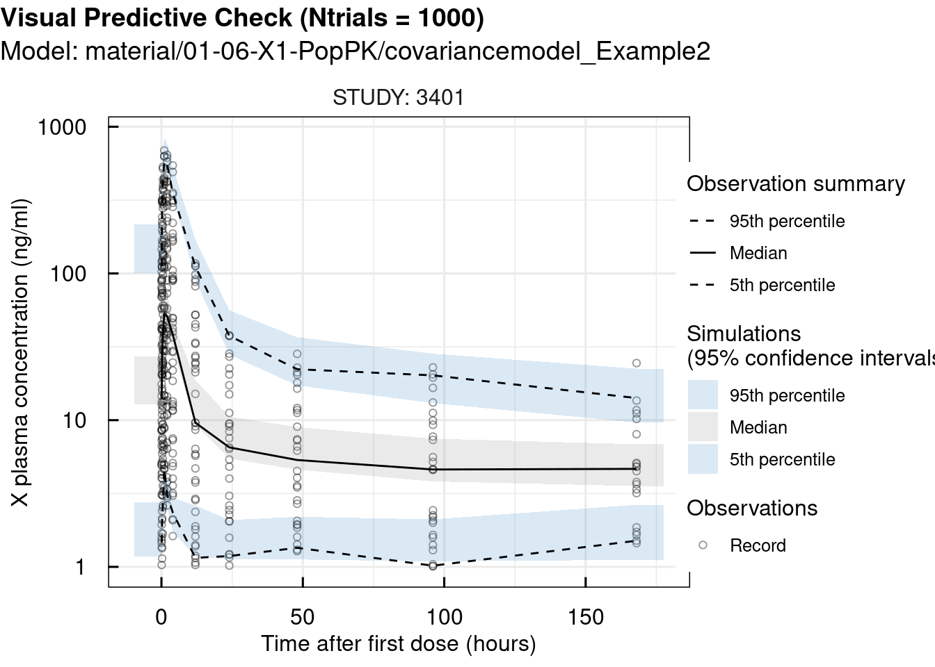
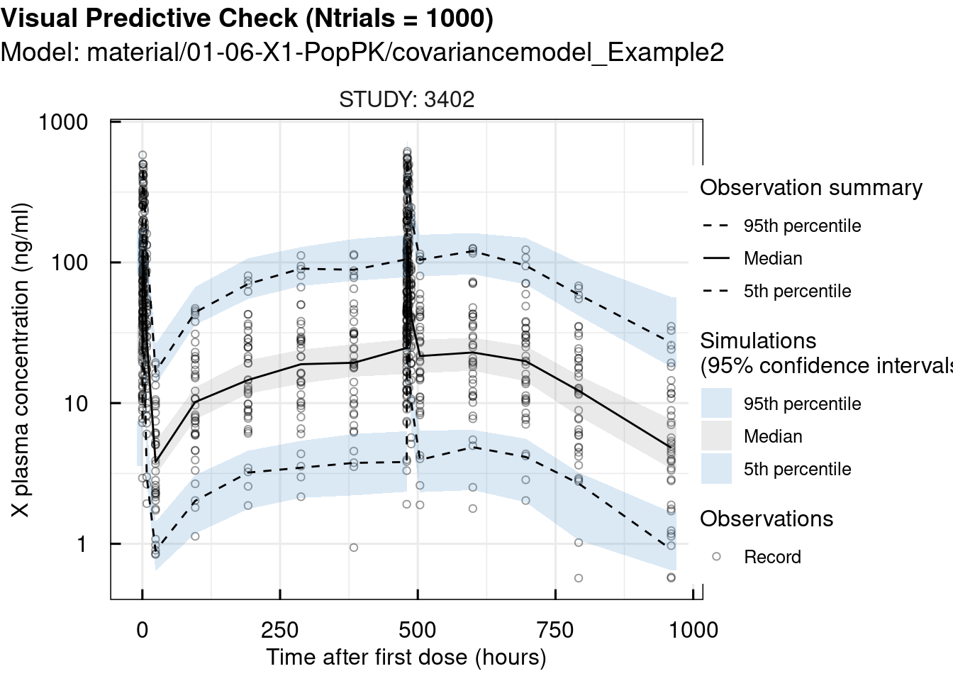
## 2 pages were printed to the graphics device.Since the observations closely match the simulations, we can conclude that the selected model is appropriate for this case.
In conclusion, from data modeling to model construction and validation, IQR Tools provided all the necessary support and tests for conducting a population pharmacokinetics (PopPK) analysis.
14.2 Reporting
Reporting can be done by IQReport (https://iqreport.intiquan.com), which allows to seemlessly integrate the results generated by IQR Tools into Word reports.