16 Experimental design
Experimental design techniques are useful to assess what type of experiments or studies should be conducted to ensure an adequate level of information in the observed data to address the question(s) of interest. In this chapter we discuss and exemplify some of these techniques.
16.1 Use of PopED
PopED is a well known optimal experimental design software that can be used both for population and individual studies based on nonlinear mixed-effect models. Methods, underlying PopED are described in Nyberg et al. (2012) and Foracchia et al. (2004). PopED is available as an R package on CRAN. The installer of IQR Tools will install the correct version automatically.
PopED comes with great flexibility for defining models and design specifications. However, the use is made overly complicated by a not well thought through R based interface to functions. The user either needs to be a PopED specialist or he/she will most likely make more or less critical mistakes, leading to wrong results and interpretations.
In order to make the important functionality of this optimal experiment design package available in a much more seamless manner, an interface between IQR Tools and PopED was developed. It benefits from the already available, intuitive, description of models and from the intuitive and easy to setup NLME model specification in IQR Tools. The user is not required to re-code models or NLME model specifications to use PopED. The same objects are used as if a user would like to perform a parameter estimation task.
The approach employed is to convert the IQR Tools model and design specifications to a PopED database. In the current version then standard PopED functions can be used on this database object. In a future version of IQR Tools dedicated functions will be provided to encapsulate the PopED functions, ensuring the easy creation of powerful and report-ready output in terms of tables and graphics.
Below an example for an IQR Tools run with PopED is given, which is based on an example model in the PopED R package. The same example is repeated in native PopED syntax. The results of both approaches are identical. The reader of this documentation can decide freely which syntax is easier to understand, review, validate, and re-use.
16.1.1 PopED / IQR Toolsinterface
We will consider a one compartment first order absorption PK model with a direct response, inhibitory IMAX, model as PD. This model in the IQRmodel syntax is available here. In a first step this model is loaded into R:
The study design to be evaluated is defined as a list with the named elements time, dosing, groupsize.
The example implements a parallel design with three arms/groups with same observation times between groups and observables. N=4 subjects per group. Each group obtains a different dose (20, 40, and placebo).
# Define study design to be evaluated
design <- list(

  # The time element defines the sampling times for the observables.
  # Here we have two observables (PK as OUTPUT1 and PD as OUTPUT2).
  # It is easily possible to define different observation times for the different outputs.
  # In this example we chose the same sampling times as in the original PopED example (even if the final
  # sampling time appears twice ... just as in the PopED example).
  time = list(
    g1 = list(OUTPUT1 = c(1, 2, 8, 240, 240),
              OUTPUT2 = c(1, 2, 8, 240, 240)),
    g2 = list(OUTPUT1 = c(1, 2, 8, 240, 240),
              OUTPUT2 = c(1, 2, 8, 240, 240)),
    g3 = list(OUTPUT1 = c(1, 2, 8, 240, 240),
              OUTPUT2 = c(1, 2, 8, 240, 240))
  ),

  # Define the dosing schedule for the different groups.
  dosing = list(
    g1 = IQRdosing(TIME = 0, ADM = 1, AMT = 20, ADDL = 10, II = 24),
    g2 = IQRdosing(TIME = 0, ADM = 1, AMT = 40, ADDL = 10, II = 24),
    g3 = IQRdosing(TIME = 0, ADM = 1, AMT =  0, ADDL = 10, II = 24)
  ),

  # Define the size of the groups
  groupsize = list(
    g1 = 4,
    g2 = 4,
    g3 = 4
  )
)
The model specification for the NLME model is defined in an identical fashion as if the user would like to generate a NONMEM, MONOLIX, or NLMIXR model with IQRtools. The modelSpec variable defined below is a list whose construction is aided by the function modelSpec_IQRest():
# Define model specifications related to the parameter, statistical, covariate model
modelSpec     <- modelSpec_IQRest(
  # Define initial guesses for the fixed effect parameters
  POPvalues0  = c(V=72.8, KA=0.25, CL=3.75,   Favail=0.9, E0=1120, IMAX=0.807, IC50=0.0993),
  # Define if a fixed effect is to be estimated (1) or not (0)
  POPestimate = c(V=1,    KA=1,    CL=1,      Favail=0,   E0=1,    IMAX=1,     IC50=1),
  # Define initial guesses for the random effects (standard deviations used - while PopED uses variances)
  IIVvalues0  = sqrt(c(V=0.09, KA=0.09, CL=0.25^2, Favail=0,   E0=0.09, IMAX=0,     IC50=0)),
  # Define if random effects are present and estimated (1), not present (0),
  # or fixed to a specified value and not estimated (2)
  IIVestimate = c(V=1,    KA=1,    CL=1,      Favail=0,   E0=1,    IMAX=0,     IC50=0),

  # By default lognormal distribution of individual parameters is assumed.
  # There are a multitude of additional optional settings which are not needed for
  # the present example.

  # Define error model and the initial guesses. In this example additive-proportional error models
  # are used for both observables.
  errorModel = list(
    OUTPUT1 = c("absrel", c(abs0=5e-6, rel0=0.04)),
    OUTPUT2 = c("absrel", c(abs0=100,  rel0=0.09))
  )
)
The IQR Tools function IQRpopEDdb() takes as required input arguments the structural model, the desired design, and the NLME model specification modelSpec and converts this information to a PopED database object.
# Run the PopED interface to establish the poped database
poped.db <- IQRpopEDdb(model = model,
                       design = design,
                       modelSpec = modelSpec)
This PopED database object then can be used with standard PopED functions. To perform model predictions, design evaluations, etc. In a soon to be available IQR Tools version proper IQR Tools functionality will be provided to simplify the evaluation of designs, etc.
# Execute standard PopED functions
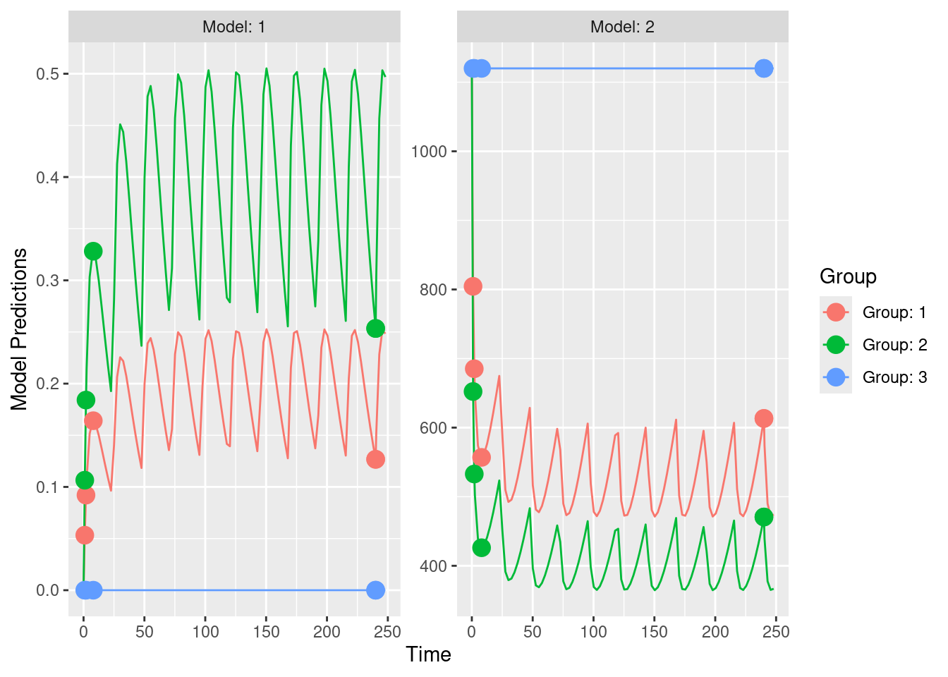
out1_IQR <- PopED::model_prediction(poped.db)
out2_IQR <- PopED::evaluate_design(poped.db)The main result of the above design evaluation are the predicted relative standard errors for the different parameters. Results for this example are shown below. The output is still fairly cryptic, as based on PopE functionality and also might require some further post-processing.
# Display the predicted relative standard errors for the parameters based on the chosen study design
print(out2_IQR$rse)
## V KA CL E0 IMAX IC50 d_V
## 18.144692 22.274798 9.626964 15.824337 22.126141 88.275210 87.071128
## d_KA d_CL d_E0
## 130.774159 57.766258 49.274222PopED results can also be plotted, using PopED functionality.
This conlcudes the example for the current IQR Tools / PopED interface. We still have some work to do to provide adequate functionality to post-process PopED output to produce reasonably nice tables and graphics that are more informative. Stay tuned … it will come in one of the next IQR Tools versions!
In the following section the same example as the one above is shown in native PopED syntax.
16.1.2 Same example in PopED
In this section, the example from the previous section, conducted with the IQR Tools interface to PopED, is performed in the native PopED syntax. The example code was taken from the examples in the PopED package on CRAN.
In a first step the model prediction function needs to be defined. This can be done using ODEs or in this case by the analytic solution. Compare this model specification to that one here. It is far easier to make a mistake in the approach below:
# Model prediction function
ff <- function(model_switch,xt,parameters,poped.db){
  with(as.list(parameters),{

    y=xt
    MS <- model_switch

    # PK model
    N = floor(xt/TAU)+1
    CONC=(DOSE*Favail/V)*(KA/(KA - CL/V)) *
      (exp(-CL/V * (xt - (N - 1) * TAU)) * (1 - exp(-N * CL/V * TAU))/(1 - exp(-CL/V * TAU)) -
         exp(-KA * (xt - (N - 1) * TAU)) * (1 - exp(-N * KA * TAU))/(1 - exp(-KA * TAU)))

    # PD model
    EFF = E0*(1 - CONC*IMAX/(IC50 + CONC))

    y[MS==1] = CONC[MS==1]
    y[MS==2] = EFF[MS==2]

    return(list( y= y,poped.db=poped.db))
  })
}
In a second step parameters and their transformation needs to be defined. For more information, please see the PopED documentation.
# Parameter definition function
sfg <- function(x,a,bpop,b,bocc){
  parameters=c( V=bpop[1]*exp(b[1]),
                KA=bpop[2]*exp(b[2]),
                CL=bpop[3]*exp(b[3]),
                Favail=bpop[4],
                DOSE=a[1],
                TAU = a[2],
                E0=bpop[5]*exp(b[4]),
                IMAX=bpop[6],
                IC50=bpop[7])
  return( parameters )
}
In a third step the residual error model function is defined. Again, the interested reader is referred to the PopED documentation for further clarification.
# Residual Error function
feps <- function(model_switch,xt,parameters,epsi,poped.db){
  returnArgs <- ff(model_switch,xt,parameters,poped.db)
  y <- returnArgs[[1]]
  poped.db <- returnArgs[[2]]

  MS <- model_switch

  pk.dv <- y*(1+epsi[,1])+epsi[,2]
  pd.dv <-  y*(1+epsi[,3])+epsi[,4]

  y[MS==1] = pk.dv[MS==1]
  y[MS==2] = pd.dv[MS==2]

  return(list( y= y,poped.db =poped.db ))
}
The create.poped.database() function in PopED then is used to combine the above information and to define the design to be evaluated.
# Create PopED database
poped.db <- PopED::create.poped.database(ff_fun="ff",
                                         fError_fun="feps",
                                         fg_fun="sfg",
                                         groupsize=4,
                                         m=3,
                                         bpop=c(V=72.8,KA=0.25,CL=3.75,Favail=0.9,E0=1120,IMAX=0.807,
                                                IC50=0.0993),
                                         notfixed_bpop=c(1,1,1,0,1,1,1),
                                         d=c(V=0.09,KA=0.09,CL=0.25^2,E0=0.09),
                                         sigma=c(0.04,5e-6,0.09,100),
                                         notfixed_sigma=c(0,0,0,0),
                                         xt=c( 1,2,8,240,240,1,2,8,240,240),
                                         minxt=c(0,0,0,240,240,0,0,0,240,240),
                                         maxxt=c(10,10,10,248,248,10,10,10,248,248),
                                         discrete_xt = list(0:248),
                                         G_xt=c(1,2,3,4,5,1,2,3,4,5),
                                         bUseGrouped_xt=1,
                                         model_switch=c(1,1,1,1,1,2,2,2,2,2),
                                         a=list(c(DOSE=20,TAU=24),c(DOSE=40, TAU=24),c(DOSE=0, TAU=24)),
                                         maxa=c(DOSE=200,TAU=40),
                                         mina=c(DOSE=0,TAU=2),
                                         ourzero=0)
Once this is completed, we execute the same functions as in the previous IQR Tools / PopED example.
# Execute standard PopED functions
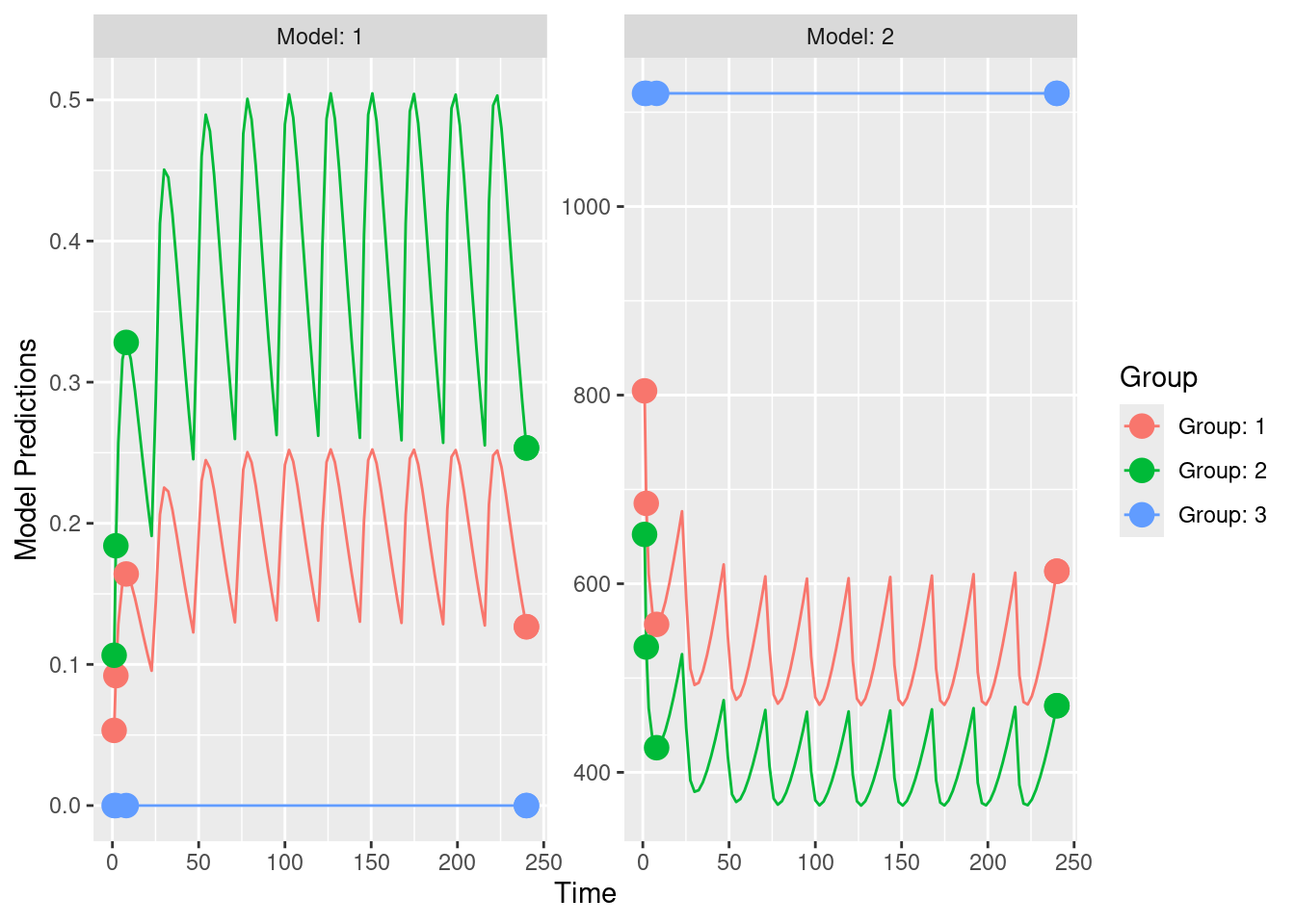
out1_IQR <- PopED::model_prediction(poped.db)
out2_IQR <- PopED::evaluate_design(poped.db)The results are basically identical to the previous example. The observed small differences stem from the fact that in this native PopED example an analytic solution was used, while in the other example the model was implemented using ordinary differential equations and the solutions to the model were integrated numerically.
# Display the predicted relative standard errors for the parameters based on the chosen study design
print(out2_IQR$rse)
## V KA CL E0 IMAX IC50 d_V
## 18.156519 22.290494 9.625457 15.824391 22.126653 88.276094 87.119440
## d_KA d_CL d_E0
## 130.861826 57.763841 49.274240Same plot as in previous example: