
12 QSP Modeling
This chapter explains how to run estimation projects using a systems pharmacology approach in IQRtools using data in IQRsysData format and an IQRmodel.
The fit is conducted in two steps with the first step consisting of the definition of an estimation object (function IQRsysEst) which is then used in a second step as an input argument for the estimation process (function IQRsysFit).
12.1 Background
Systems Biology and Systems Pharmacology strive to enhance the understanding of biogical systems by describing their dynamic behavior with mechanistic models. The models are often complex as they represent, e.g., networks of signaling events or metabolic pathways. Efficient parameters estimation algorithms are required for this type of models. Using tools implemented for NLME modeling in Pharmacometrics are often not suited for these complex models (and not appropriate for non-NLME models) typically used for Systems Pharmacology.
IQRtools implements a parameter estimation approach based on trust region optimization of the negative log-likelihood utilizing symbolically derived sensitivities to improve numerical robustness 1,2.
Combined with the option of multiple estimation starting points it aims at identifying the globally best solution.
In addition, it enables the combination of many experimental conditions in one objective function to facilitate fitting a model to diverse data.
The parameters can therefore be estimated for all and/or selected experimental conditions.
Furthermore, the estimation of the profile likelihood provides information about overall parameter identifiability by calculating confidence intervals.
This results in a powerful and fast parameter estimation tool delivering robust parameter estimates.
12.2 Interface
The interface of the IQRtools QSP toolbox is designed to resemble the IQRtools NLME interface.
Additionally to the two-stage approach of setting up estimation objects via IQRsysEst() which converted into parameter estimation projects via IQRsysProject(), a new object called IQRsysModel is introduced in order to complete the cycle of model building/ model refinement, parameter estimation and model assessment.
The most simple form of an IQRsysModel contains just the structural model, specified as IQRmodel.
As in IQRnlme, a comprehensive model description of the current modelling task can be constructed by the four arguments model dosing, data and modelSpec in order to account for dosing, covariates and even inter-individual variability (IIV).
The majority of features in IQRnlme are also implemented in IQRsys, plus some QSP-specific features such as condition-specific parameters.
Below is a short summary of the differences compared to IQRnlme (better as table)
12.2.1 Data
- An additional column in the data sheed called CONDITION is required. CONDITION contains identifiers of the respective experimental conditions.
12.2.2 ModelSpec
- (not yet) supported fields
covarianceModelis by default “diagonal” and cannot be changed in IQRsysEstPriorVarPOP,PriorVarCovariateModelValues,PriorVarErrorModel,PriorIIV,PriorDFIIVare not supported on IQRsysEst-level but can be supplied in IQRsysProject
- Additional fields (for condition-specific (“local”) parameters)
LOCmodelLOCvalues0LOCestimateLOCdistribution
(For IQRsysModel, a few other features are allowed, such a list of IQRdosings for the dosing-argument, but for a first start, this might be too confusing??)
12.3 Systems Biology Example: Epo-Receptor
The following example model was published by Becker et al., 2010 describing information processing at the Epo receptor. A cartoon of the model can be seen in Figure x.
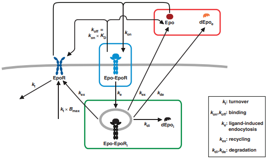
The IQRmodel-representation of the model is given by
********** MODEL NAME

Becker et al

********** MODEL NOTES

The model by Becker et al. (2010) shows that
rapid EpoR turnover and large intracellular receptor
pools enables linear ligand response.

********** MODEL STATES

d/dt(Epo)          = initEpo*INPUT1 + EpoEpoRi*kex + EpoEpoR*koff - Epo*EpoR*kon
d/dt(EpoR)       = EpoEpoRi*kex + EpoEpoR*koff - EpoR*kt + 4*initEpo*initEpoRrel*kt - Epo*EpoR*kon
d/dt(EpoEpoR)      = Epo*EpoR*kon - EpoEpoR*koff - EpoEpoR*ke
d/dt(EpoEpoRi)   = EpoEpoR*ke - EpoEpoRi*kdi - EpoEpoRi*kde - EpoEpoRi*kex
d/dt(dEpoi)      = EpoEpoRi*kdi
d/dt(dEpoe)      = EpoEpoRi*kde

Epo(0)           = 0
EpoR(0)          = 4*initEpo*initEpoRrel
EpoEpoR(0)       = 0
EpoEpoRi(0)      = 0
dEpoi(0)         = 0
dEpoe(0)         = 0


********** MODEL PARAMETERS

initEpo = 1350
initEpoRrel = 0.09
kD = 142
kde =   0.012
kdi = 0.0013
ke = 0.055
kex = 0.00058
koff = 0.081
kon = 0.15
kt = 0.016
offset = 1e-5
scale   = 0.98

********** MODEL VARIABLES

Epoext = Epo + dEpoe
Epoint = EpoEpoRi + dEpoi

Epoextcpm = log10(offset + (Epoext*scale)/initEpo)
Epomemcpm = log10(offset + (EpoEpoR*scale)/initEpo)
Epointcpm = log10(offset + (Epoint*scale)/initEpo)

OUTPUT1 = Epoextcpm
OUTPUT2 = Epomemcpm
OUTPUT3 = Epointcpm


********** MODEL REACTIONS


********** MODEL FUNCTIONS


********** MODEL EVENTS
12.3.1 Basic model simulation
The most simple way to define an IQRsysModel is to pass an IQRmodel without any additional specifications. As such, it can already be simulated and plotted.
sysModel <- IQRsysModel("material/01-04b-BasicQSPmodeling/Example1_Epo/Scripts/Resources/model.txt")
sysModel <- sim_IQRsysModel(sysModel)
plot_IQRsysModel(sysModel)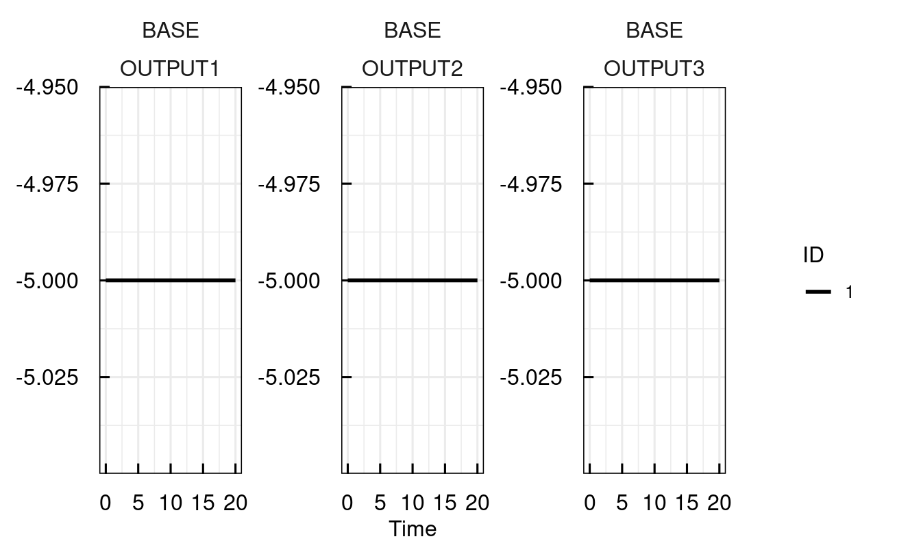
To obtain a feeling for the model behaviour, let us invoke the model with an IQRdosing, which in this case represents a bolus of Epo at t = 0.
sysModel <- IQRsysModel("material/01-04b-BasicQSPmodeling/Example1_Epo/Scripts/Resources/model.txt",
                        dosing = IQRdosing(TIME = 0, ADM = 1, AMT = 1))
sysModel <- sim_IQRsysModel(sysModel)
plot_IQRsysModel(sysModel)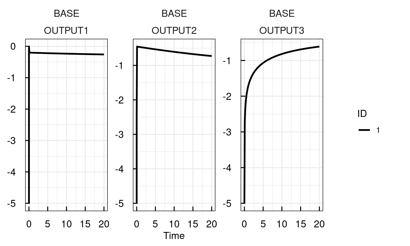
Simulating the model with sim_IQRsysModel returns the same IQRsysModel with updated simulations.
In order to store these results, the results have to be reassigned.
sysModel <- sim_IQRsysModel(sysModel, simtime = 1:300, FLAGoutputsOnly = FALSE)
sysModel <- sim_IQRsysModel(sysModel)
plot_IQRsysModel(sysModel)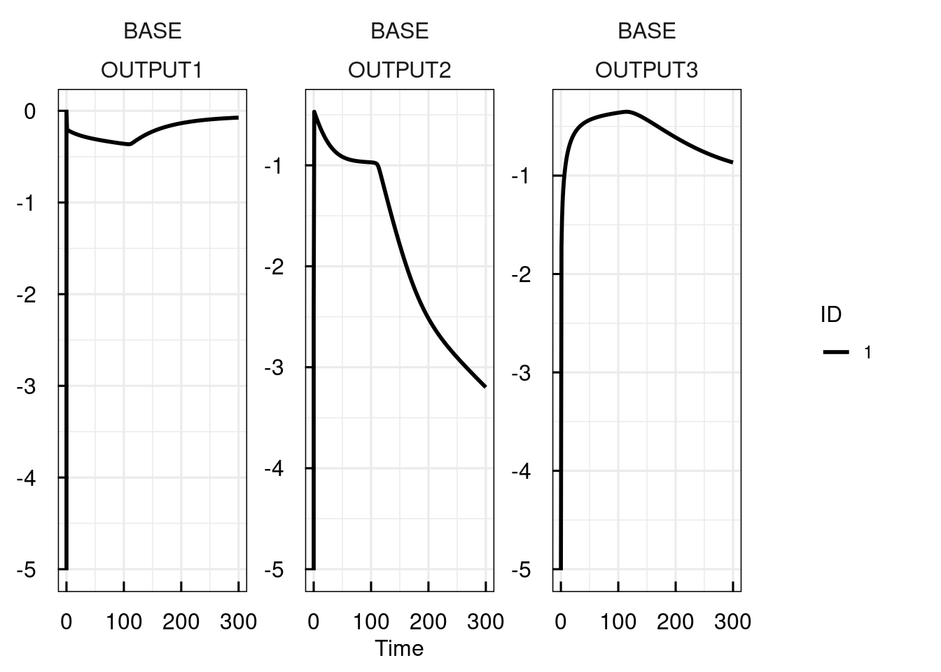
12.3.2 Manipulating parameters for simulations
Viewing and manipulating model parameters is facilitated by the functions getPars_IQRsysModel() and setPars_IQRsysModel().
For example, first we print a comprehensive list of available parameters and then update the parameter kon to the value kon = 0.2, simulate and plot the new model predictions.
sysModel <- IQRsysModel("material/01-04b-BasicQSPmodeling/Example1_Epo/Scripts/Resources/model.txt",
                        dosing = IQRdosing(TIME = 0, ADM = 1, AMT = 1))
pars <- getPars_IQRsysModel(sysModel) # aside from printing the parameter-table, a nemd vector of parameters is returned
## --- Selected optimum: --------------------------------## --- Global parameters ---------------------------------## --- No local parameters defined -----------------------## Parameter | Value | Estimate
## --------------------------------------
## | |
## **Error model** | |
## | |
## error_ADD1 | 1 | +L
## error_ADD2 | 1 | +L
## error_ADD3 | 1 | +L
## | |
## **Fixed effects** | |
## | |
## initEpo | 1350 | -
## initEpoRrel | 0.09 | -
## kde | 0.012 | -
## kdi | 0.0013 | -
## ke | 0.055 | -
## kex | 0.00058 | -
## koff | 0.081 | -
## kon | 0.15 | -
## kt | 0.016 | -
## offset | 1e-05 | -
## scale | 0.98 | -
##
## Values rounded to 4 significant digits.
## Estimated/fixed parameters (+/-)
## Estimation on (N) natural / (L) log / (G) logit scale.sysModel <- setPars_IQRsysModel(sysModel, kon = 0.01)
sysModel <- sim_IQRsysModel(sysModel, 1:300, FLAGoutputsOnly = TRUE)
plot_IQRsysModel(sysModel)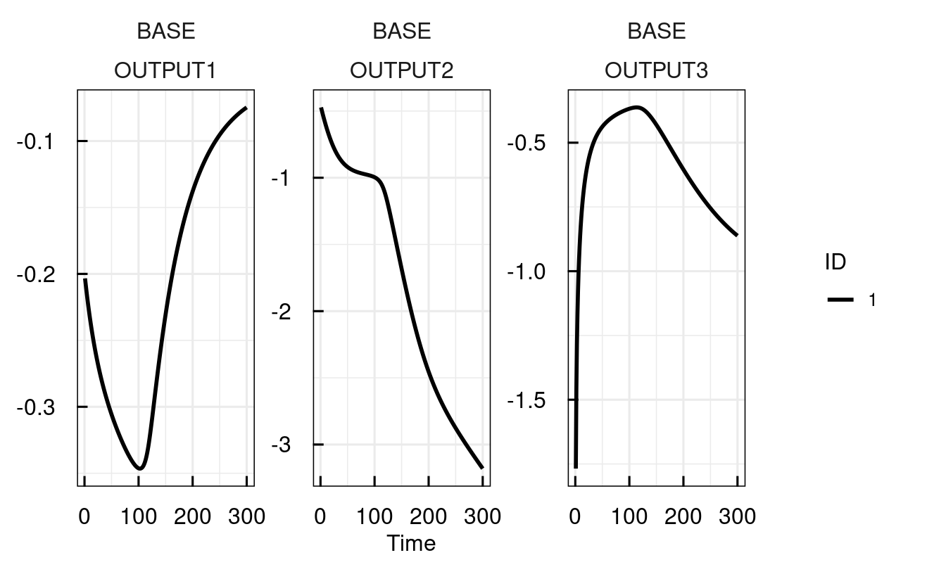
Alternatively, parameters can be directly supplied to sim_IQRsysModel
plot_IQRsysModel(sim_IQRsysModel(sysModel,
                                 1:300,
                                 parameters =  c(kon = 0.15, ke = 0.0001),
                                 FLAGoutputsOnly = TRUE))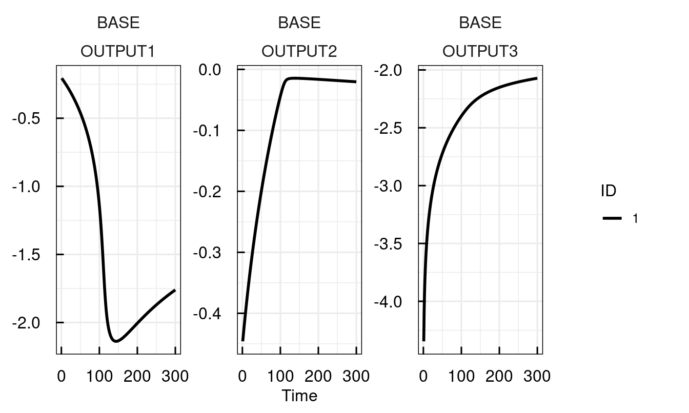
12.3.3 Defining experimental conditions
Different experimental conditions are encoded in IQRsysModel via the LOC...-fields in modelSpec.
LOC stands for local parameters, i.e. condition specific parameters.
Here, we define two different experimental conditions with different initial Epo-concentrations in the Petri-dish.
LOCmodelis a named list with the following structure:list(parametername = c("condition1", "condition2")). It can be omitted, ifLOCvalues0is provided.LOCvalues0is a list with the following structurelist(parametername = c("condition1" = value1, "condition2" = value2)).LOCestimateuses the same number code asPOPestimate, 0 = fixed (default), 1 = estimate,.LOCdistributionuses the same code as IIVdistribution."L"= log-scale (default),"N"= linear scale,"G"= logit-scale
mspec <-  modelSpec_IQRsysEst(
  POPvalues0 = c(
    kon   = 0.2,
    kt    = 0.1,
    scale = 1
  ),
  LOCmodel = list(
    initEpo = c("EpoLow", "EpoHigh")
  ),
  LOCvalues0 = list(
    initEpo = c(EpoLow = 500, EpoHigh = 1500)
  ),
  LOCestimate = list(
    initEpo = c(EpoLow = 0, EpoHigh = 0)
  )
)

sysModel <- IQRsysModel(
  model = "material/01-04b-BasicQSPmodeling/Example1_Epo/Scripts/Resources/model.txt",
  modelSpec = mspec,
  dosing = IQRdosing(TIME = 0, ADM = 1, AMT = 1)
)
getPars_IQRsysModel(sysModel)
## --- Selected optimum: --------------------------------## --- Global parameters ---------------------------------## Parameter | Value | Estimate
## --------------------------------------
## | |
## **Error model** | |
## | |
## error_ADD1 | 1 | +L
## error_ADD2 | 1 | +L
## error_ADD3 | 1 | +L
## | |
## **Fixed effects** | |
## | |
## kon | 0.2 | +L
## kt | 0.1 | +L
## scale | 1 | +L
## initEpoRrel | 0.09 | -
## kde | 0.012 | -
## kdi | 0.0013 | -
## ke | 0.055 | -
## kex | 0.00058 | -
## koff | 0.081 | -
## offset | 1e-05 | -## --- Local parameters ----------------------------------## Parameter | Value | Estimate | Condition
## ------------------------------------------------
## | | |
## **Fixed effects** | | |
## | | |
## initEpo_EpoLow | 500 | - | EpoLow
## initEpo_EpoHigh | 1500 | - | EpoHigh
##
## Values rounded to 4 significant digits.
## Estimated/fixed parameters (+/-)
## Estimation on (N) natural / (L) log / (G) logit scale.The two parameters initEpo_EpoLow and initEpo_EpoHigh have been created to reflect the condition specificity. These parameters can also be accessed or modified by setPars_IQRsysModel and sim_IQRsysModel:
plot_IQRsysModel(sim_IQRsysModel(sysModel,
                                 simtime = 1:500,
                                 parameters = c(initEpo_EpoLow = 10)), FLAGerror = FALSE)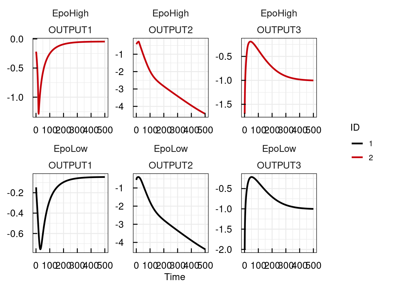
Selecting parameters with condition-specific values returns all instances of this parameter:
##             kon             kde  initEpo_EpoLow initEpo_EpoHigh
##         2.0e-01         1.2e-02         5.0e+02         1.5e+03
12.3.4 Modeling data - exploration by manual parameter tweaking
First construct the IQRsysModel with specifying the data-argument.
# Importing as an IQRsysData object imputes some columns
dataSys <- import_IQRsysData("material/01-04b-BasicQSPmodeling/Example1_Epo/Data/dataRAW.csv")
write.csv(dataSys, "material/01-04b-BasicQSPmodeling/Example1_Epo/Data/dataSYS.csv")

# Load the model, dataSYS.csv
sysModel <- IQRsysModel("material/01-04b-BasicQSPmodeling/Example1_Epo/Scripts/Resources/model.txt",
                        data = list(datafile = "material/01-04b-BasicQSPmodeling/Example1_Epo/Data/dataSYS.csv"))
sysModel <- sim_IQRsysModel(sysModel)
print(sysModel)
## --- IQRsysModel object - basic information: -----------##
## Model: material/01-04b-BasicQSPmodeling/Example1_Epo/Scripts/Resources/model.txt
## Dosing: No dosing.
## Data: material/01-04b-BasicQSPmodeling/Example1_Epo/Data/dataSYS.csv
## Specs: No model specification
##
## Conditions: Experiment_1## --- Additional information stored: --------------------##
## Multistart estimation results: no
## Profile likelihood analysis: no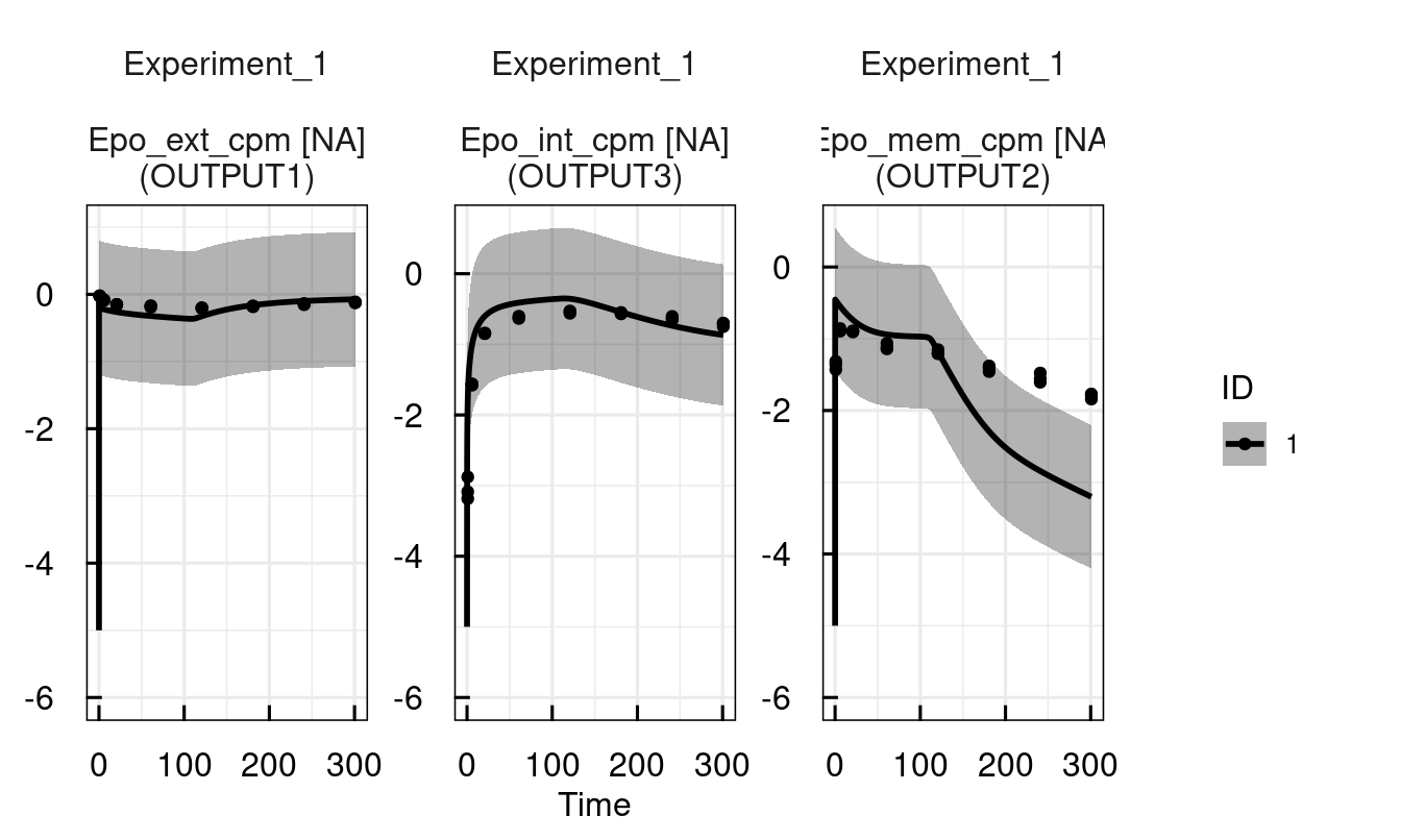
# Manual parameter tweaking
# Reduce error parameters
sysModel <- setPars_IQRsysModel(sysModel,
error_ADD1 = 0.1,
error_ADD2 = 0.1,
error_ADD3 = 0.1)
sysModel <- sim_IQRsysModel(sysModel, simtime = 1:300)
plot(sysModel)
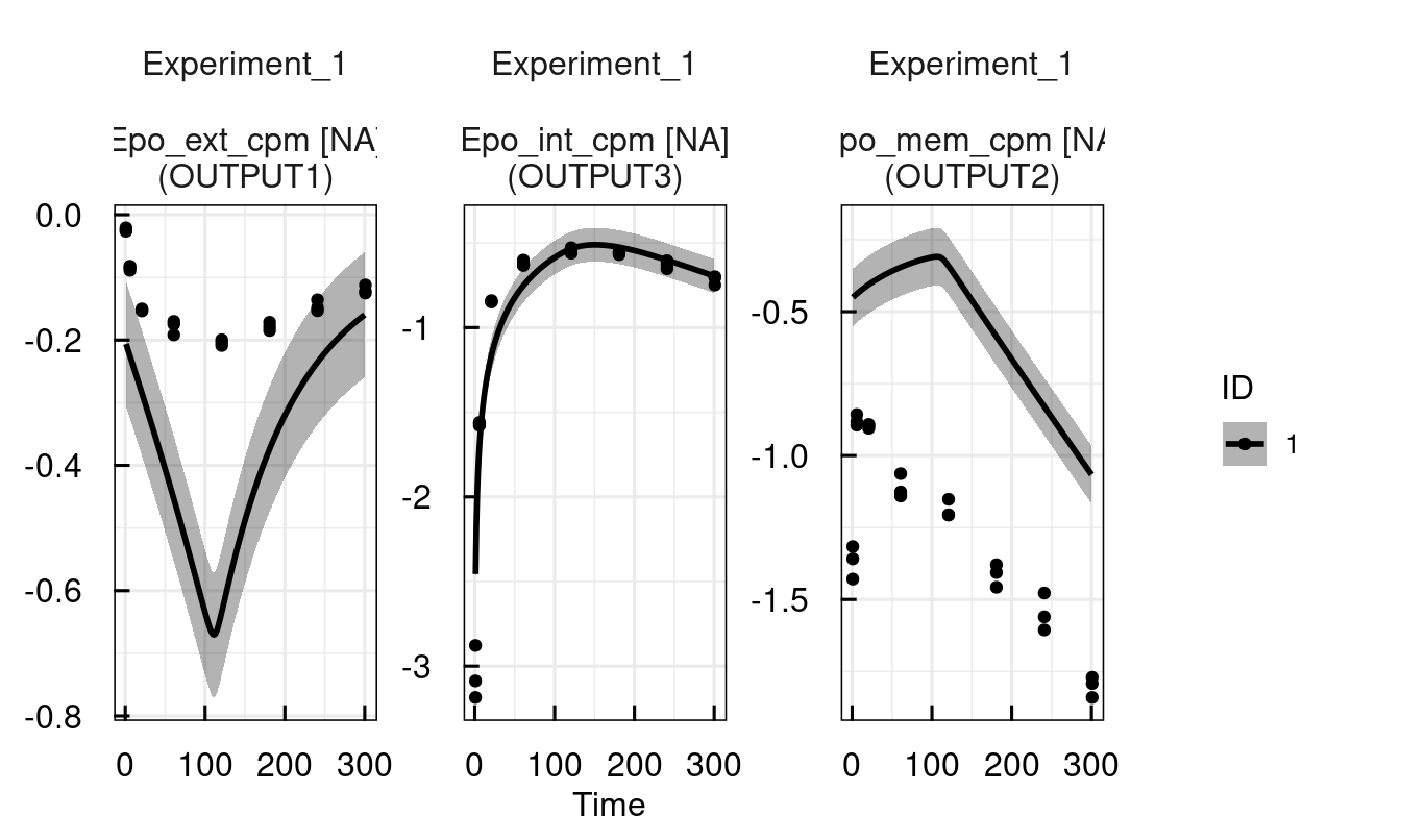
# Decrease endocytosis rate to retain more EpoR on the membrane
sysModel <- setPars_IQRsysModel(sysModel, ke = 0.01)
sysModel <- sim_IQRsysModel(sysModel, simtime = 1:300)
plot(sysModel)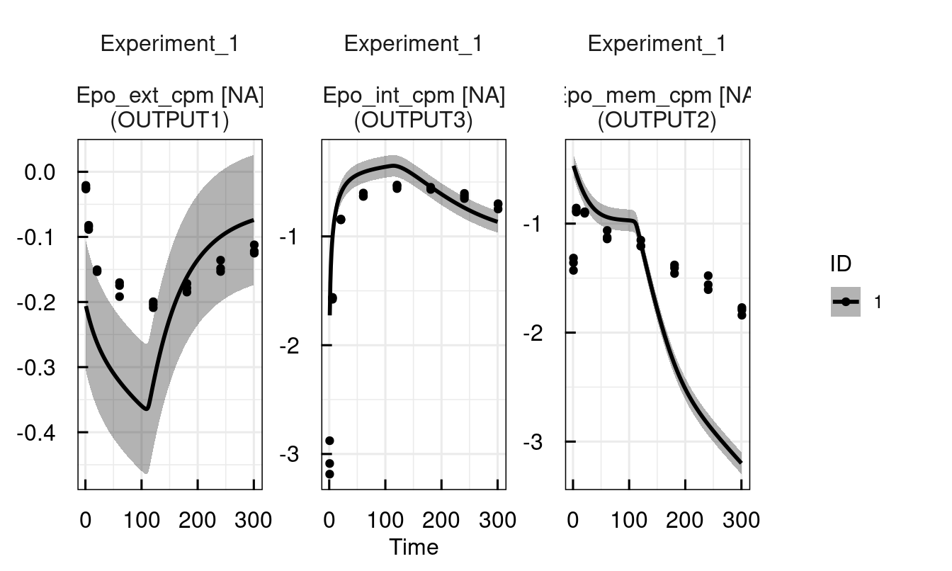
12.3.5 Modeling data - parameter estimation
If an IQRsysModel object (containing data) exists, this can readily be converted to an estimation object by as_IQRsysEst
sysModel <- IQRsysModel("material/01-04b-BasicQSPmodeling/Example1_Epo/Scripts/Resources/model.txt",
                        data = list(datafile = "material/01-04b-BasicQSPmodeling/Example1_Epo/Data/dataSYS.csv"))

# Convert to estimation object
est <- as_IQRsysEst(
  sysModel,
  modelSpec = list(
    POPestimate = c(
      initEpoRrel = 1,
      kde         = 1,
      kdi         = 1,
      ke          = 1,
      kex         = 1,
      koff        = 1,
      kon         = 1,
      kt          = 1
    )
  ))
Another option is to specify the estimation object from the basic objects itself:
# Convert to estimation object
est <- IQRsysEst(
  model = "material/01-04b-BasicQSPmodeling/Example1_Epo/Scripts/Resources/model.txt",
  dosing = list(INPUT1=c(type = "BOLUS")),
  data = list(datafile = "material/01-04b-BasicQSPmodeling/Example1_Epo/Data/dataSYS.csv"),
  modelSpec = modelSpec_IQRsysEst(
    POPvalues0 = c(
      initEpoRrel = 0.09,
      kde         = 0.12,
      kdi         = 0.0013,
      ke          = 0.01,
      kex         = 0.00058,
      koff        = 0.081,
      kon         = 0.15,
      kt          = 0.016
    ),
    POPestimate = c(
      initEpoRrel = 1,
      kde         = 1,
      kdi         = 1,
      ke          = 1,
      kex         = 1,
      koff        = 1,
      kon         = 1,
      kt          = 1
    )
  ))
The next step is to run the specified parameter estimation by creating an IQRsysProject and then running it.
Running the IQRsysProject does two things: It outputs all results to the specified folder, including GOF plots, standardized report-ready tables, etc. On the other hand, the result of run_IQRsysProject is yet again an IQRsysModel with updated parameter estimation information!
Therefore, we can continue analysing the model right away once the computations are finished.
# Create sysProject
proj <- IQRsysProject(est, "material/01-04b-BasicQSPmodeling/Example1_Epo/Models/RUN1", opt.nfits = 4)

# Run project and return result as optimized sysModel
sysModel <- run_IQRsysProject(proj, FLAGgof = FALSE)

# Inspect estimated parameters and fit
sysModel <- sim_IQRsysModel(sysModel, simtime = 1:300)
plot_IQRsysModel(sysModel)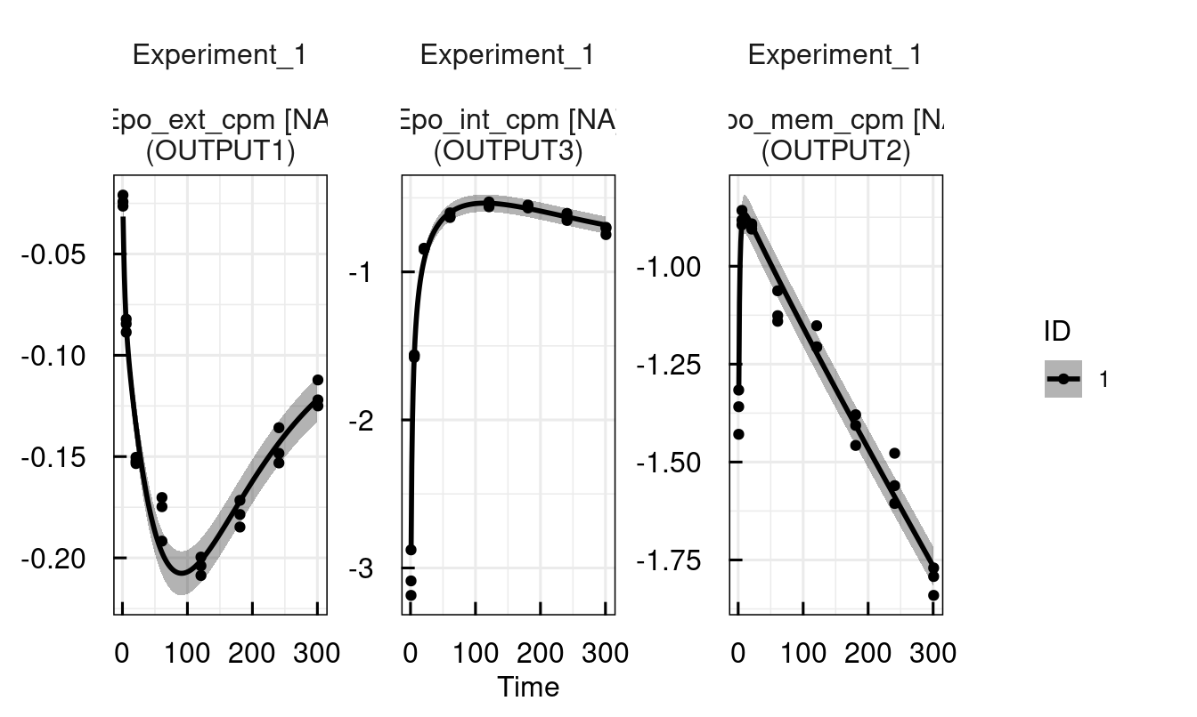
If the work should be resumed later, the function load_IQRsysProject loads the sysModel stored in the project folder.
## Warning: Project result not available. Might lead to problems in recompilation## Rebuilding IQRsysModel ...
##
## Convert data to dMod ...... done.
## Convert model to basic dMod model ..... done.
## Link basic dMod model to data ...... done.
##
## ... successful.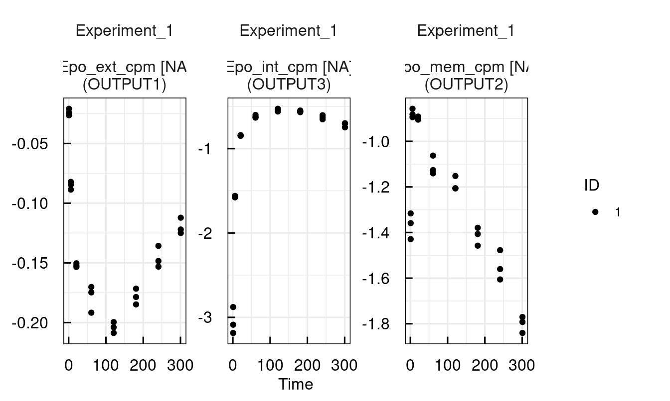
12.3.6 Modeling data - multistart optimization
sysModel <- IQRsysModel("material/01-04b-BasicQSPmodeling/Example1_Epo/Scripts/Resources/model.txt",
data = list(datafile = "material/01-04b-BasicQSPmodeling/Example1_Epo/Data/dataSYS.csv"))
# Convert to estimation object
est <- as_IQRsysEst(
sysModel,
modelSpec = list(
POPestimate = c(
initEpoRrel = 1,
kde = 1,
kdi = 1,
ke = 1,
kex = 1,
koff = 1,
kon = 1,
kt = 1
)
))
# Run optimizations
proj <- IQRsysProject(est, "material/01-04b-BasicQSPmodeling/Example1_Epo/Models/RUN2",
opt.nfits = 36, opt.sd = 3)
sysModel <- run_IQRsysProject(proj, ncores = 8)
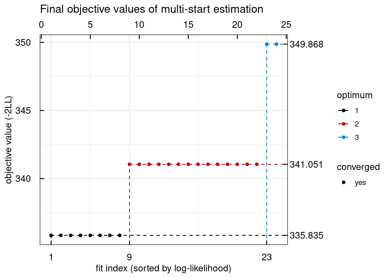
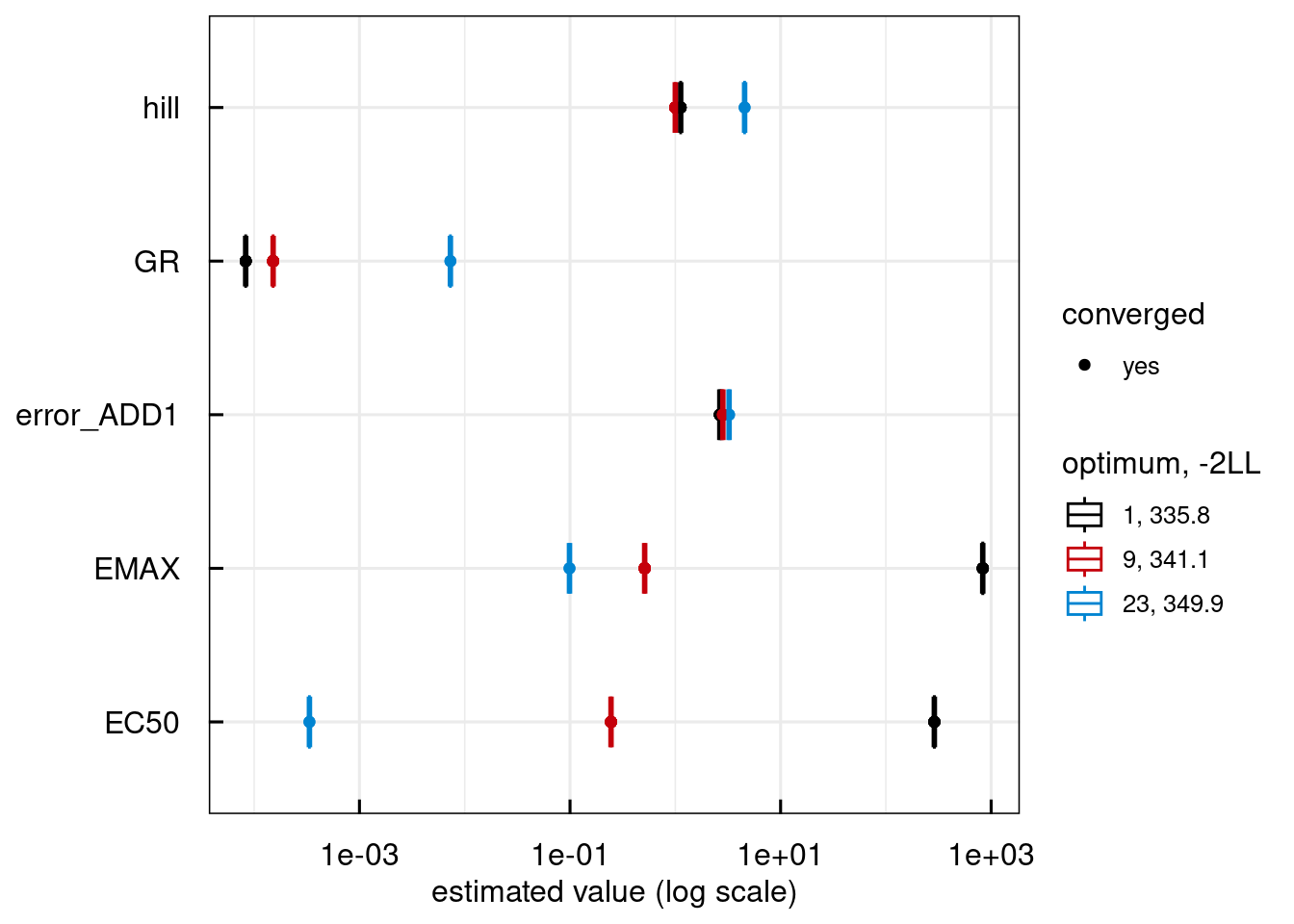
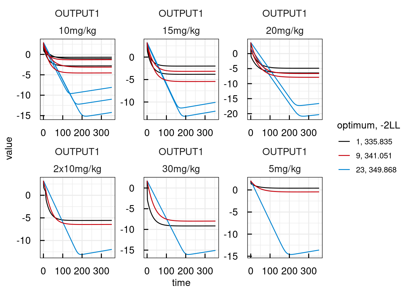
# Exploring the results of the multi-start estimation
plotWaterfall_IQRsysModel(sysModel)
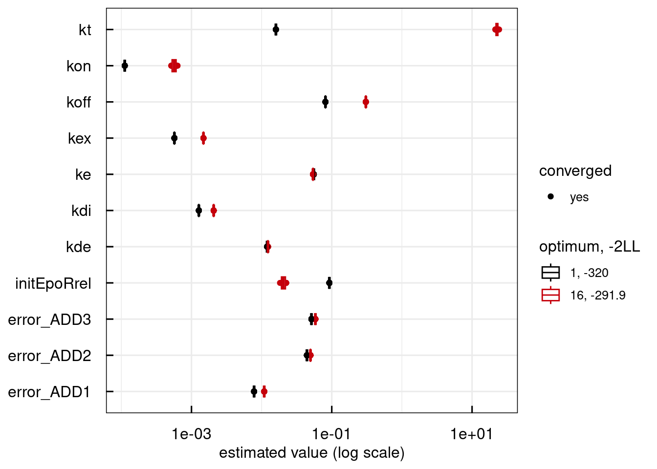
plotPars_IQRsysModel(sysModel)
plotPred_IQRsysModel(sysModel)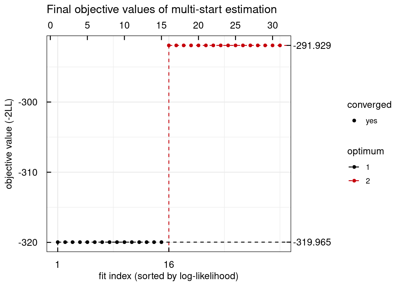
## Warning: Parameter vector of an unconverged fit is selected.
## Warning: Parameter vector of an unconverged fit is selected.
## Warning: Parameter vector of an unconverged fit is selected.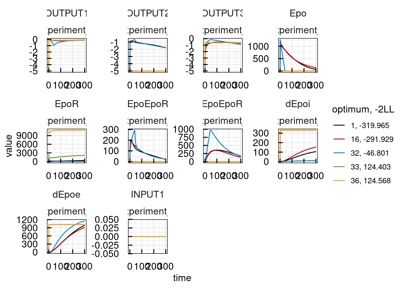
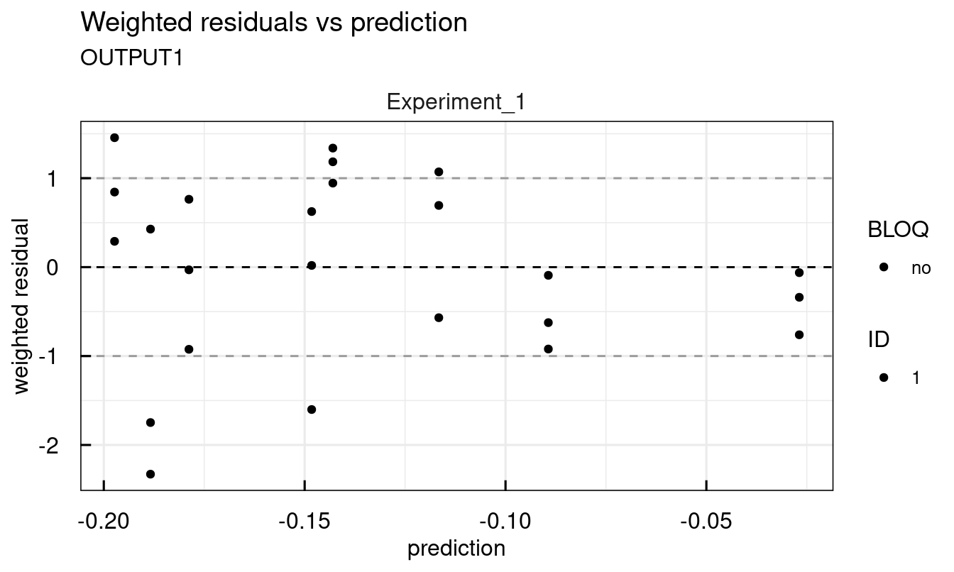
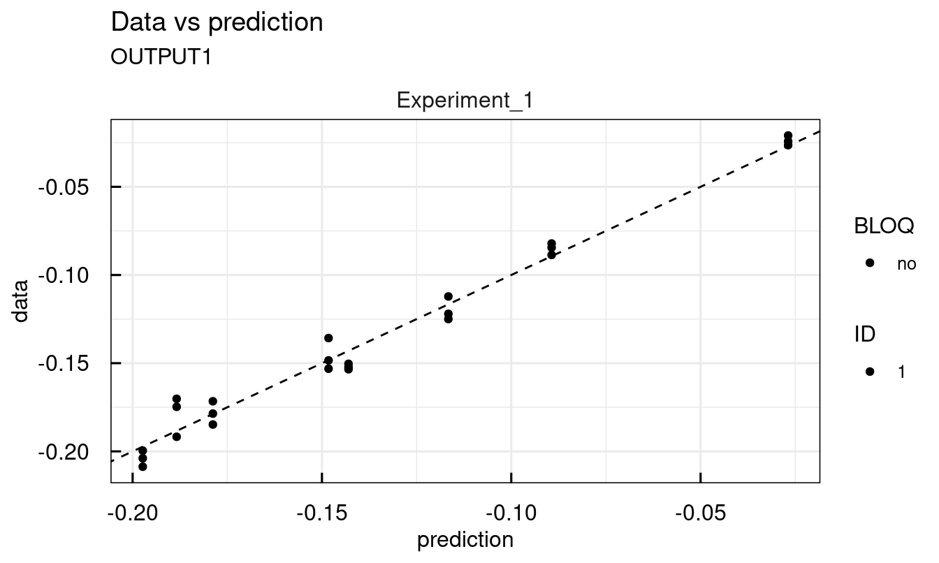
Other available plots are found at the end of the description of each plotting function ?plot_IQRsysModel in the See Also section. For example, standard diagnostic plots:
## 2 page output has been printed.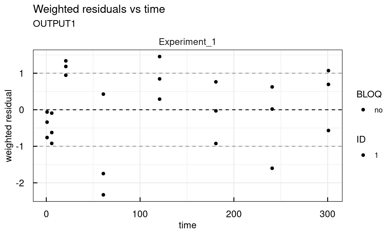
12.3.7 Modeling data - Profile Likelihood
In non-linear parameter estimation problems, confidence intervals from the Fisher Information are often deceiving, since the Log-Likelihood is only poorly approximated by a quadratic Taylor expansion. The Profile Likelihood however was shown to yield the correct confidence intervals for much weaker assumptions. IQRsys offers functionality to compute the profile likelihoods of the estimated parameters via a sophisticated and fast integration-based algorithm.
Profiles can be either directly computed when an IQRsysProject is created and executed or they can be added later via the profile_IQRsysModel function.
sysModel <- IQRsysModel("material/01-04b-BasicQSPmodeling/Example1_Epo/Scripts/Resources/model.txt",
                        data = list(datafile = "material/01-04b-BasicQSPmodeling/Example1_Epo/Data/dataSYS.csv"))

# Convert to estimation object
est <- as_IQRsysEst(
  sysModel,
  modelSpec = list(
    POPestimate = c(
      initEpoRrel = 1,
      kde         = 1,
      kdi         = 1,
      ke          = 1,
      kex         = 1,
      koff        = 1,
      kon         = 1,
      kt          = 1
    )
  ))

# Run optimizations and profile Likelihood
proj <- IQRsysProject(est, "material/01-04b-BasicQSPmodeling/Example1_Epo/Models/RUN3",
                      opt.nfits = 36, opt.sd = 3,
                      FLAGprofileLL = TRUE
                      )
sysModel <- run_IQRsysProject(proj, ncores = 24)

# Plot profile likelihood information
plotProfile_IQRsysModel(sysModel)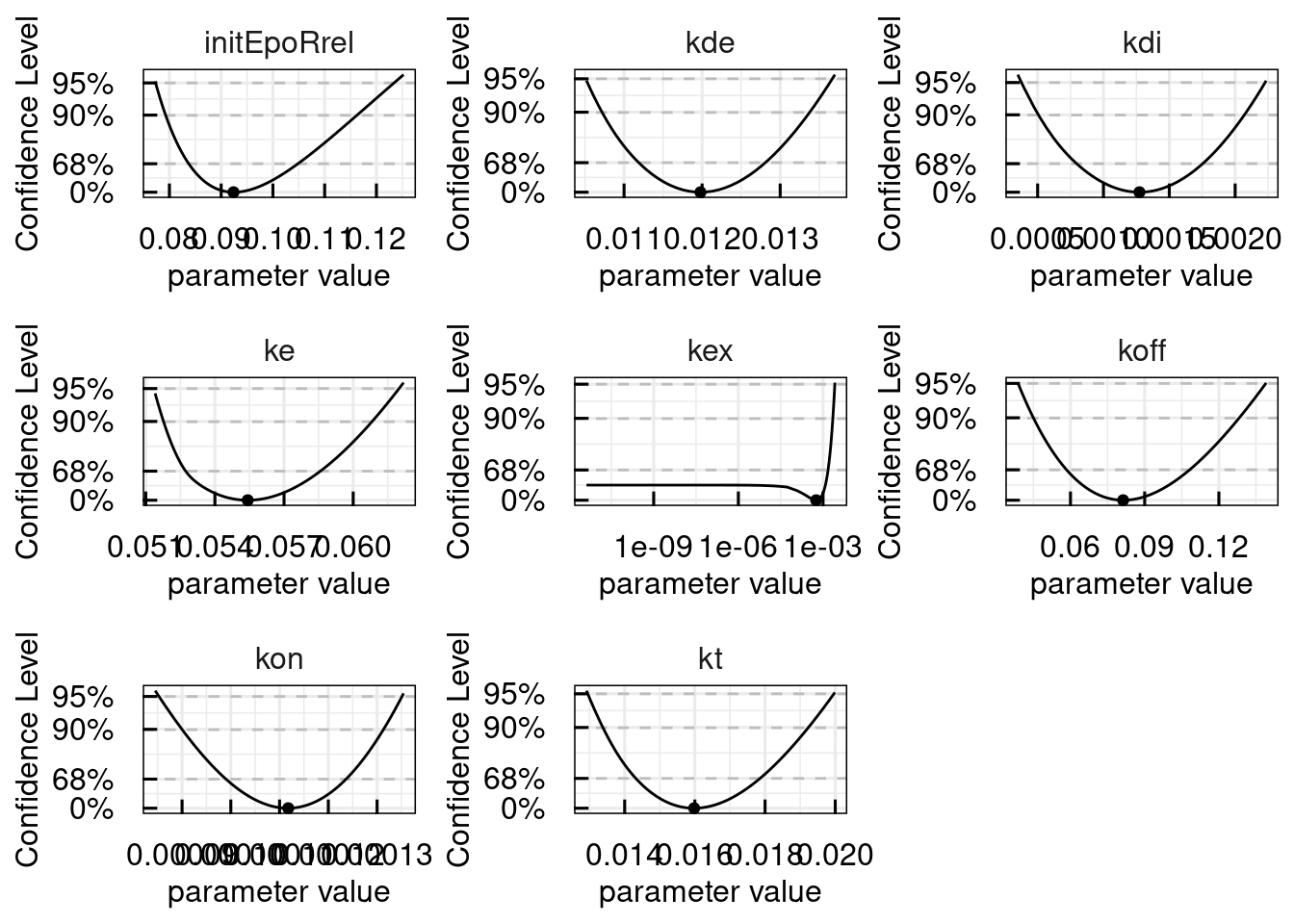
We see, that the parameter kex is practically non-identifiable, which is characterized by an infinitely large confidence interval, but with a unique optimum in the profile likelihood.
Such non-identifiabilities can be resolved either by more informative data or by model-reduction, which will be added to the IQRtools documentation soon.
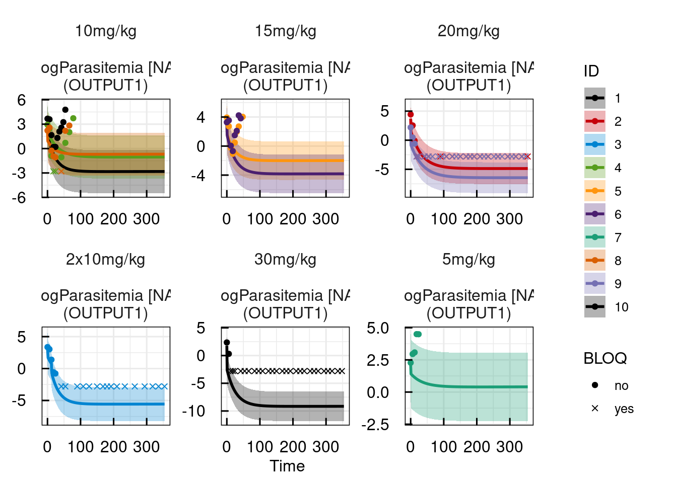
12.3.8 Modelling data - IIV and BLOQ (censored data)
The next example showcases two additional features of IQRsys, handling of IIV and handling of left-censored data, e.g. data below the limit of quantification (BLOQ).
The ability to handle IIV with the same syntax as in IQRnlme was a key point in the design of the IQRsys-interface.
IIV is specified in the modelSpec as shown in the IQRnlme description.
Data points BLOQ are handled by default with the likelihood absed approach as described in Beal, method M3. Options to use other methods such as M4 are in current development.
As a comparison, we first demonstrate fitting the model without IIV, then with IIV:
# Setting up sysModel object with data and model specification
sysmodel <- IQRsysModel(
# Model
model = "material/01-04b-BasicQSPmodeling/Example2_Malaria/Scripts/Resources/model.txt",
# Data
data = list(
datafile = "material/01-04b-BasicQSPmodeling/Example2_Malaria/Data/data.csv",
regressorNames = c("Fabs1", "ka", "CL", "Vc",
"Q1", "Vp1", "Tlag1", "PLbase")
),
# Specs
modelSpec = list(
POPvalues0 = c(PLerr = 0 , GR = 0.02,
EMAX = 0.1, EC50 = 0.01, hill = 4 ),
POPestimate = c(PLerr = 0 , GR = 1 ,
EMAX = 1 , EC50 = 1 , hill = 1 ),
IIVdistribution = c(PLerr ='N', GR ='L' ,
EMAX ='L' , EC50 ='L' , hill ='L'),
errorModel = list(
OUTPUT1 = c(type = "abs", guess = 1)
)
)
)
sysmodel <- sim_IQRsysModel(sysmodel)
plot(sysmodel)
# Estimate population parameters
est <- as_IQRsysEst(sysmodel)
proj <- IQRsysProject(est,
projectPath = "material/01-04b-BasicQSPmodeling/Example2_Malaria/Models/01_NoIIV",
opt.nfits = 24,
opt.sd = 2,
opt.parupper = c(hill = 10),
opt.parlower = c(hill = 1))
suppressMessages(optsys <- run_IQRsysProject(proj, ncores = 8, FLAGgof = FALSE))
# Plot best fit
plot(optsys)
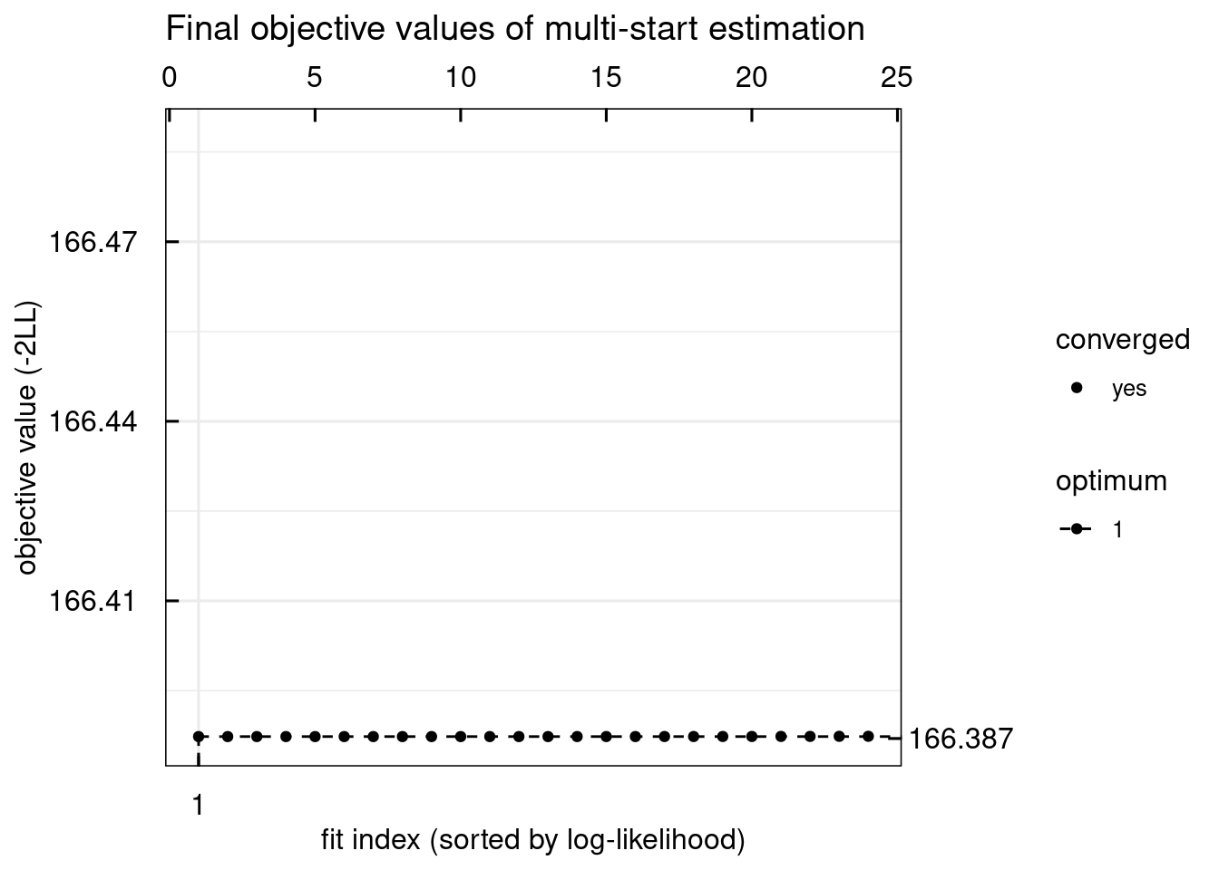
plotWaterfall_IQRsysModel(optsys)
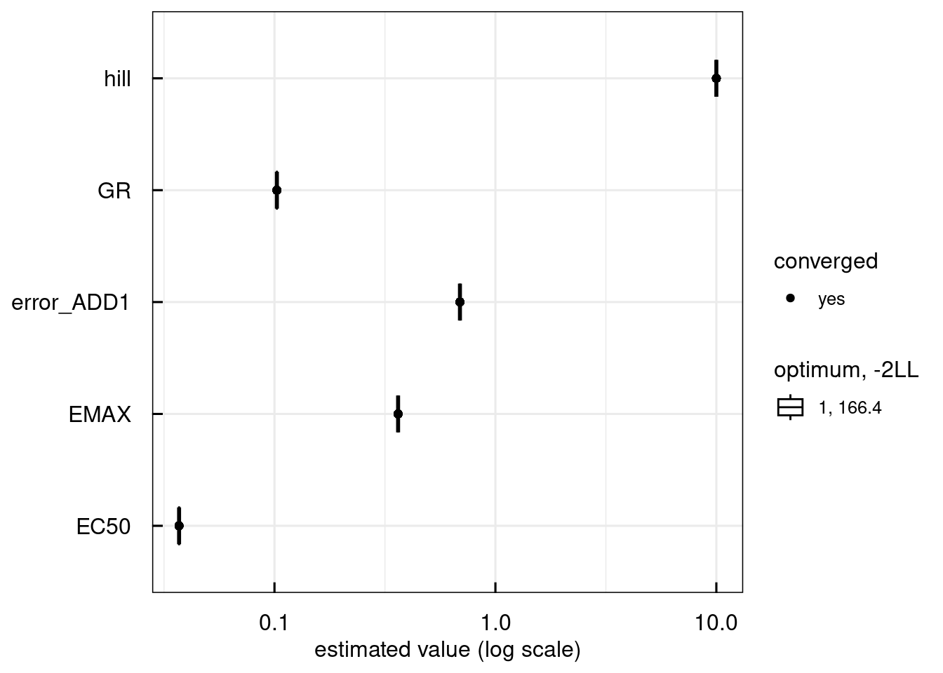
plotPars_IQRsysModel(optsys)
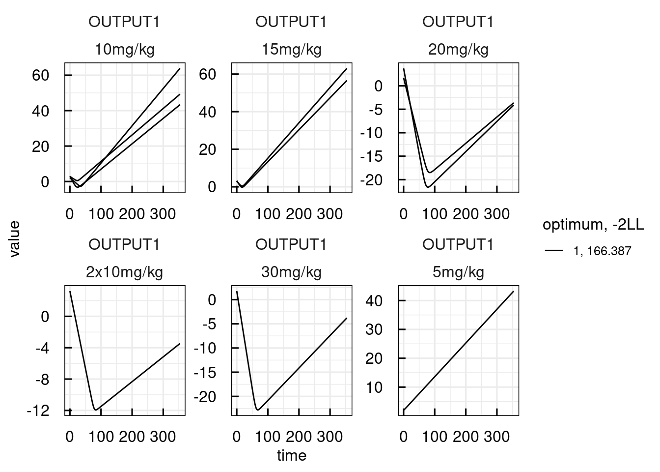
plotPred_IQRsysModel(optsys, states = "OUTPUT1")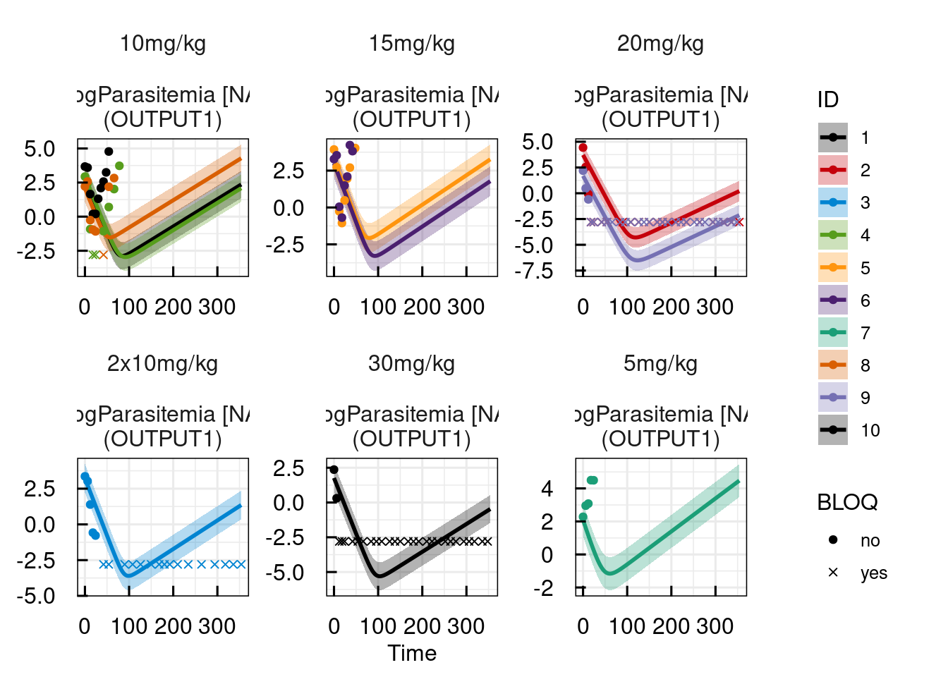
# Setting up sysModel object with data and model specification
sysmodel <- IQRsysModel(
  # Model
  model = "material/01-04b-BasicQSPmodeling/Example2_Malaria/Scripts/Resources/model.txt",
  # Data
  data  = list(
    datafile = "material/01-04b-BasicQSPmodeling/Example2_Malaria/Data/data.csv",
    regressorNames = c("Fabs1", "ka", "CL", "Vc",
                       "Q1", "Vp1", "Tlag1", "PLbase")
  ),
  # Specs
  modelSpec = list(
    POPvalues0      = c(PLerr = 0 , GR = 0.02,
                        EMAX = 0.1, EC50 = 0.01, hill = 4 ),
    POPestimate     = c(PLerr = 0 , GR = 1   ,
                        EMAX = 1  , EC50 = 1   , hill = 1 ),
    IIVdistribution = c(PLerr ='N', GR ='L'  ,
                        EMAX ='L' , EC50 ='L'  , hill ='L'),
    IIVvalues0      = c(GR = 0.5, EMAX = 0.5, EC50 = 0.5),
    IIVestimate     = c(GR = 2  , EMAX = 2  , EC50 = 2  ),
    errorModel = list(
      OUTPUT1 = c(type = "abs", guess = 1)
    )
  )
)

# Estimate population parameters + IIV
est <- as_IQRsysEst(sysmodel)

proj <- IQRsysProject(est,
                      projectPath = "material/01-04b-BasicQSPmodeling/Example2_Malaria/Models/02_IIV",
                      opt.nfits = 24,
                      opt.sd = 2,
                      opt.parupper = c(hill = 10),
                      opt.parlower = c(hill = 1))

suppressMessages(optsys <- run_IQRsysProject(proj, ncores = 8, FLAGgof = TRUE))

plot(optsys)

plotWaterfall_IQRsysModel(optsys)
plotPars_IQRsysModel(optsys)
plotPred_IQRsysModel(optsys, states = "OUTPUT1")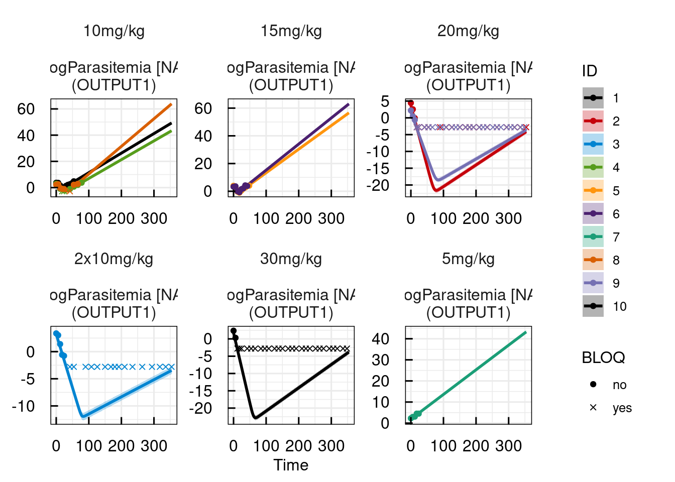
Raue, Bioinformatics 31(21), 2015↩︎
Kaschek, dMod, 2016 (https://cran.r-project.org/package=dMod)↩︎